Competition Perfect competition is an industry in which

Competition Perfect competition is an industry in which: – Many firms sell identical products to many buyers. Each buys or sells only a tiny fraction of the total quantity in the market. – Sellers can easily enter into or exit from market. – Established firms have no advantages over new ones. – Sellers and buyers are well informed about prices. – Sellers offer a standardized product. 1

Competition Perfect competition arises: – When firm’s minimum efficient scale is small relative to market demand so there is room for many firms in the industry. – And when each firm is perceived to produce a good or service that has no unique characteristics, so consumers don’t care which firm they buy from. 2

Competition • Price Takers – In perfect competition, each firm is a price taker. – A price taker is a firm that cannot influence the price of a good or service. – No single firm can influence the price—it must “take” the equilibrium market price. – Each firm’s output is a perfect substitute for the output of the other firms, so the demand for each firm’s output is perfectly elastic. 3

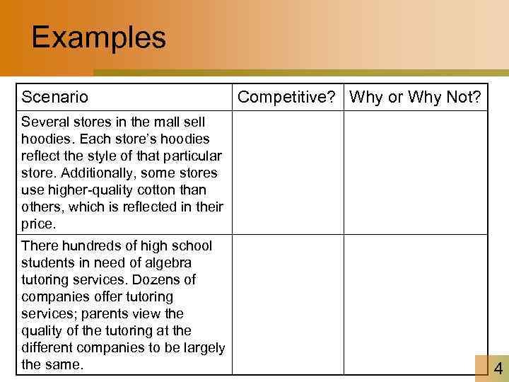Examples Scenario Competitive? Why or Why Not? Several stores in the mall sell hoodies. Each store’s hoodies reflect the style of that particular store. Additionally, some stores use higher-quality cotton than others, which is reflected in their price. There hundreds of high school students in need of algebra tutoring services. Dozens of companies offer tutoring services; parents view the quality of the tutoring at the different companies to be largely the same. 4

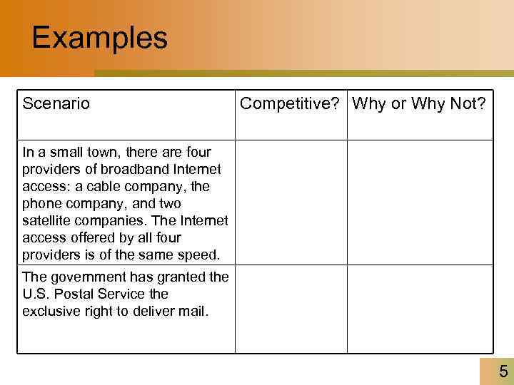Examples Scenario Competitive? Why or Why Not? In a small town, there are four providers of broadband Internet access: a cable company, the phone company, and two satellite companies. The Internet access offered by all four providers is of the same speed. The government has granted the U. S. Postal Service the exclusive right to deliver mail. 5

Competition • Economic Profit and Revenue – The goal of each firm is to maximize economic profit, which equals total revenue minus total cost. – Total cost is the opportunity cost of production, which includes normal profit. – A firm’s total revenue equals price, P, multiplied by quantity sold, Q, or P Q. – A firm’s marginal revenue is the change in total revenue that results from a one-unit increase in the quantity sold. 6

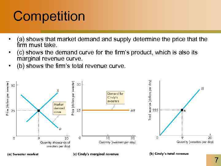Competition • (a) shows that market demand supply determine the price that the firm must take. • (c) shows the demand curve for the firm’s product, which is also its marginal revenue curve. • (b) shows the firm’s total revenue curve. 7

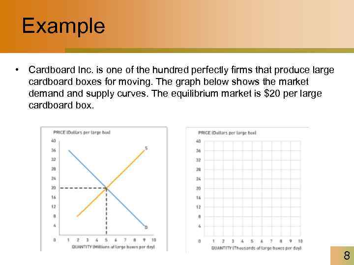Example • Cardboard Inc. is one of the hundred perfectly firms that produce large cardboard boxes for moving. The graph below shows the market demand supply curves. The equilibrium market is $20 per large cardboard box. 8

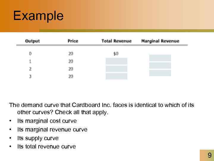Example The demand curve that Cardboard Inc. faces is identical to which of its other curves? Check all that apply. • Its marginal cost curve • Its marginal revenue curve • Its supply curve • Its total revenue curve 9

The Firm’s Decisions in Perfect Competition A perfectly competitive firm faces two constraints: • A market constraint summarized by the market price and the firm’s revenue curves • A technology constraint summarized by firm’s product curves and cost curves 10

The Firm’s Decisions in Perfect Competition – The perfectly competitive firm makes two decisions in the short run: • Whether to produce or to shut down. • If the decision is to produce, what quantity to produce. – A firm’s long-run decisions are: • Whether to stay in the industry or leave it. • Whether to increase or decrease its plant size. 11

Profit-Maximizing Output • A perfectly competitive firm chooses the output that maximizes its economic profit. • At each output level, subtract total cost from total revenue to get total profit at that output level • Total Profit = TR - TC 12

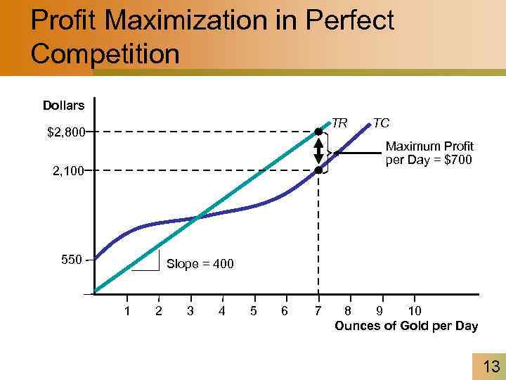Profit Maximization in Perfect Competition Dollars TR $2, 800 TC Maximum Profit per Day = $700 2, 100 550 Slope = 400 1 2 3 4 5 6 7 8 9 10 Ounces of Gold per Day 13

The Marginal Revenue and Marginal Cost Approach • Firm should continue to increase output as long as marginal revenue > marginal cost • Profit-maximizing output is found where MC curve crosses MR curve from below 14

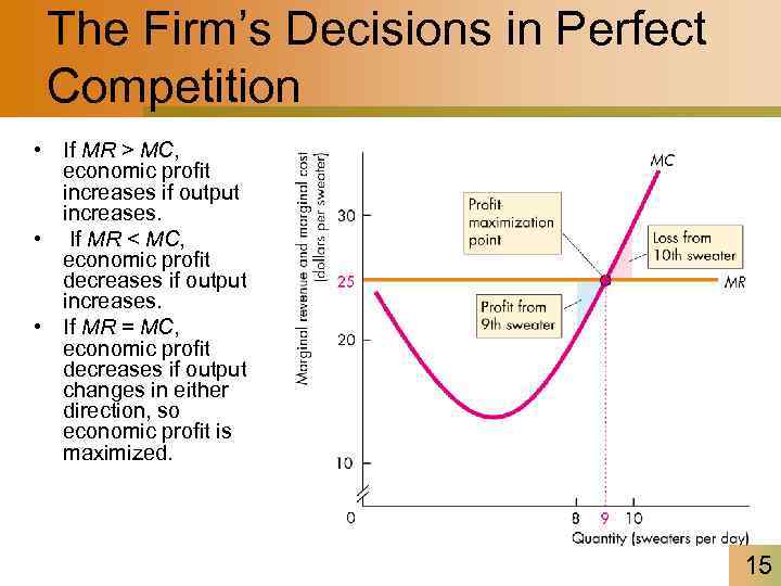The Firm’s Decisions in Perfect Competition • If MR > MC, economic profit increases if output increases. • If MR < MC, economic profit decreases if output increases. • If MR = MC, economic profit decreases if output changes in either direction, so economic profit is maximized. 15

The Firm’s Decisions in Perfect Competition • Profits and Losses in the Short Run – Maximum profit is not always a positive economic profit. – To determine whether a firm is earning an economic profit or incurring an economic loss, we compare the firm’s average total cost, ATC, at the profit maximizing output with the market price. 16

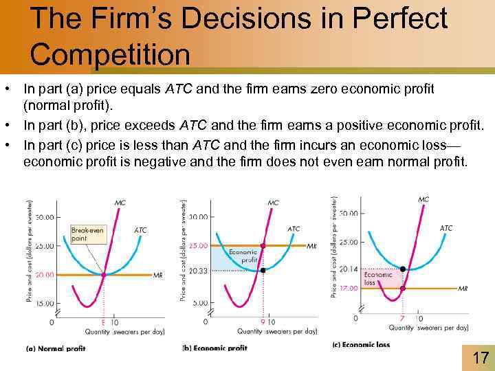The Firm’s Decisions in Perfect Competition • In part (a) price equals ATC and the firm earns zero economic profit (normal profit). • In part (b), price exceeds ATC and the firm earns a positive economic profit. • In part (c) price is less than ATC and the firm incurs an economic loss— economic profit is negative and the firm does not even earn normal profit. 17

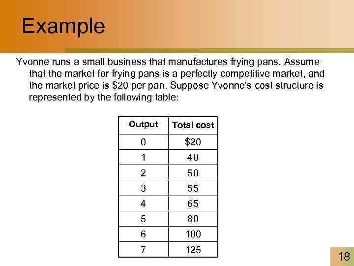Example Yvonne runs a small business that manufactures frying pans. Assume that the market for frying pans is a perfectly competitive market, and the market price is $20 per pan. Suppose Yvonne’s cost structure is represented by the following table: Output Total cost 0 $20 1 40 2 50 3 55 4 65 5 80 6 100 7 125 18

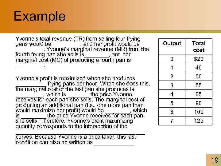Example Yvonne’s total revenue (TR) from selling four frying pans would be _____, and her profit would be _____. Yvonne’s marginal revenue (MR) from the fourth frying pan she sells is____, and her marginal cost (MC) of producing a fourth pan is _____. Yvonne’s profit is maximized when she produces _____ frying pans per hour. When she does this, the marginal cost of the last pan she produces is _____, which is _______ the price Yvonne receives for each pan she sells. The marginal cost of producing an additional pan (i. e. , one more pan than would maximize her profit) would be ____, which is ____ the price Yvonne receives for each pan she sells. Therefore, Yvonne’s profit maximizing quantity corresponds to the intersection of the _____________________ curves. Because Yvonne is a price taker, this last condition can also be written as _______ Output Total cost 0 $20 1 40 2 50 3 55 4 65 5 80 6 100 7 125 19

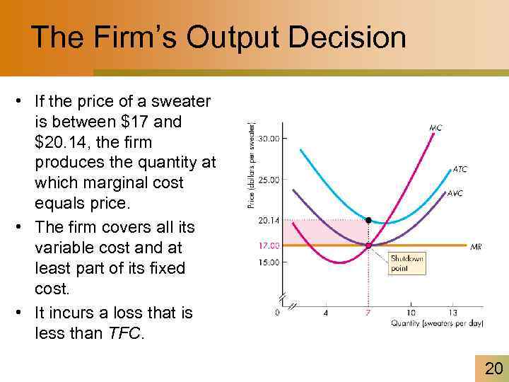The Firm’s Output Decision • If the price of a sweater is between $17 and $20. 14, the firm produces the quantity at which marginal cost equals price. • The firm covers all its variable cost and at least part of its fixed cost. • It incurs a loss that is less than TFC. 20

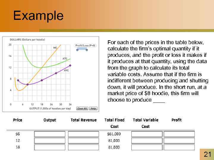Example For each of the prices in the table below, calculate the firm’s optimal quantity if it produces, and the profit or loss it makes if it produces at that quantity, using the data from the graph to calculate its total variable costs. Assume that if the firm is indifferent between producing and shutting down, it will produce. In the short run, at a market price of $8 hoodie, this firm will choose to produce ____ 21

Short-Run Supply Under Perfect Competition • The Shutdown Price: price at which a firm is indifferent between producing and shutting down • Can summarize all of this information in a single curve— firm’s supply curve – Tells us how much output the firm will produce at any price • Supply curve has two parts – For all prices above minimum point on its AVC curve, supply curve coincides with MC curve – For all prices below minimum point on AVC curve, firm will shut down – For all prices below the shutdown price output is zero and the supply curve coincides with vertical axis 22

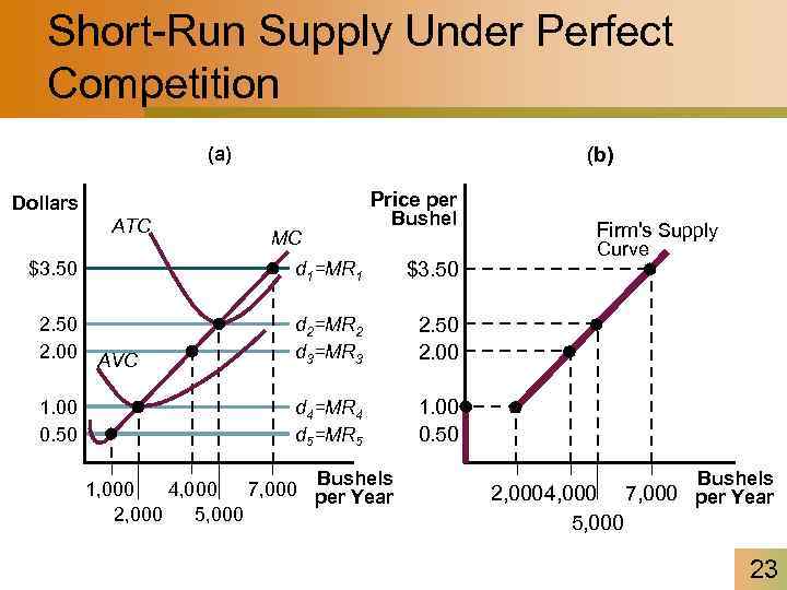Short-Run Supply Under Perfect Competition (a) (b) Price per Dollars ATC MC Bushel d 1=MR 1 $3. 50 2. 00 AVC d 2=MR 2 d 3=MR 3 d 4=MR 4 d 5=MR 5 Curve 2. 50 2. 00 1. 00 0. 50 Firm's Supply 1. 00 0. 50 $3. 50 Bushels 1, 000 4, 000 7, 000 per Year 2, 000 5, 000 2, 0004, 000 5, 000 Bushels 7, 000 per Year 23

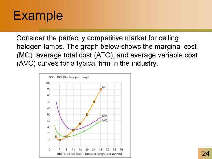Example Consider the perfectly competitive market for ceiling halogen lamps. The graph below shows the marginal cost (MC), average total cost (ATC), and average variable cost (AVC) curves for a typical firm in the industry. 24

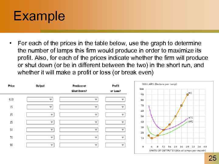Example • For each of the prices in the table below, use the graph to determine the number of lamps this firm would produce in order to maximize its profit. Also, for each of the prices indicate whether the firm will produce or shut down (or be in different between the two) in the short run, and whether it will make a profit or loss (or break even) 25

Competitive Markets in the Short. Run • Short-run is a time period too short for firm to vary all of its inputs – Quantity of at least one input remains fixed – In short-run, number of firms in industry is fixed • To determine the short-run market supply curve • amount of output that all sellers in market will offer at each price – sum quantities of output supplied by all firms in market at each price 26

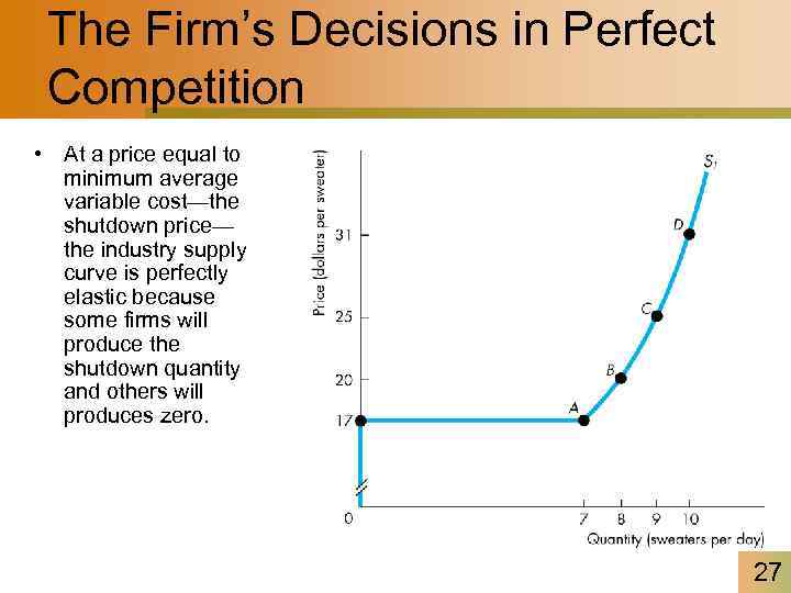The Firm’s Decisions in Perfect Competition • At a price equal to minimum average variable cost—the shutdown price— the industry supply curve is perfectly elastic because some firms will produce the shutdown quantity and others will produces zero. 27

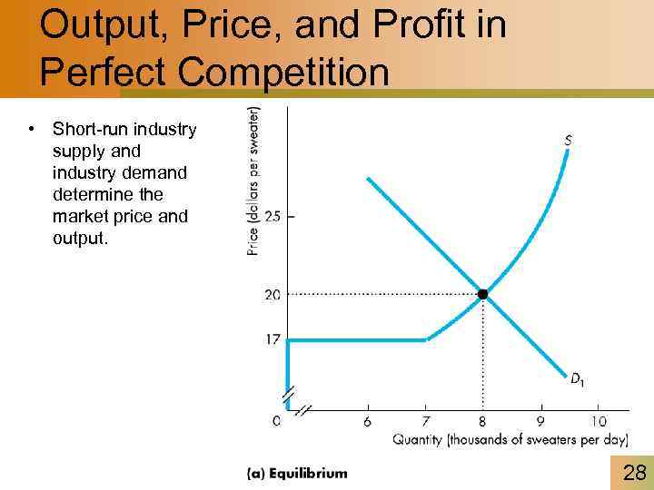Output, Price, and Profit in Perfect Competition • Short-run industry supply and industry demand determine the market price and output. 28

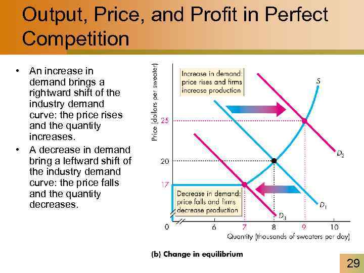Output, Price, and Profit in Perfect Competition • An increase in demand brings a rightward shift of the industry demand curve: the price rises and the quantity increases. • A decrease in demand bring a leftward shift of the industry demand curve: the price falls and the quantity decreases. 29

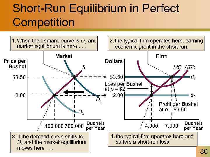Short-Run Equilibrium in Perfect Competition 1. When the demand curve is D 1 and market equilibrium is here. . . Price per Bushel Market 2. the typical firm operates here, earning economic profit in the short run. Dollars Firm S MC ATC $3. 50 2. 00 D 1 d 1 $3. 50 Loss per Bushel at p = $2 2. 00 d 2 Profit per Bushel at p = $3. 50 D 2 Bushels 400, 000 700, 000 per Year 3. If the demand curve shifts to D 2 and the market equilibrium moves here. . . 4, 000 7, 000 Bushels per Year 4. the typical firm operates here and suffers a short-run loss. 30

Output, Price, and Profit in Perfect Competition • Long-Run Adjustments – In short-run equilibrium, a firm may earn an economic profit, earn normal profit, or incur an economic loss and which of these states exists determines the further decisions the firm makes in the long run. – In the long run, the firm may: • Enter or exit an industry • Change its plant size 31

From Short-Run Profit to Long-Run Equilibrium • Economic profit will attract new entrants • Increasing number of firms in market – As number of firms increases, market supply curve will shift rightward » Market price begins to fall » As market price falls, demand curve facing each firm shifts downward » Each firm—striving as always to maximize profit—will slide down its marginal cost curve, decreasing output 32

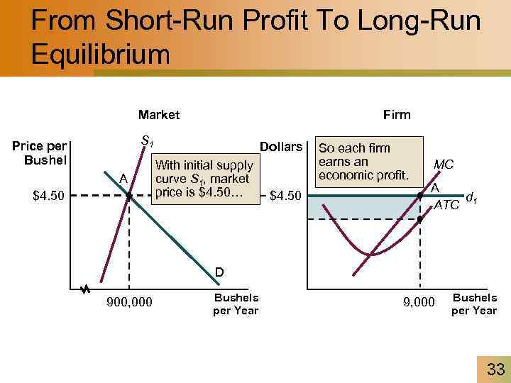From Short-Run Profit To Long-Run Equilibrium Market Firm S 1 Price per Bushel A $4. 50 Dollars With initial supply curve S 1, market price is $4. 50… $4. 50 So each firm earns an economic profit. MC A d ATC 1 D 900, 000 Bushels per Year 9, 000 Bushels per Year 33

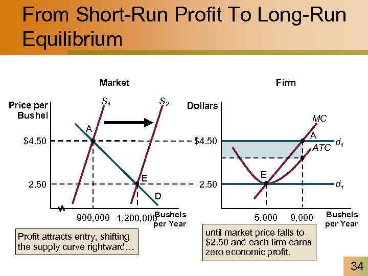From Short-Run Profit To Long-Run Equilibrium Market Firm S 1 Price per Bushel S 2 Dollars MC A $4. 50 A d ATC 1 $4. 50 E 2. 50 E d 1 D Bushels 900, 000 1, 200, 000 per Year Profit attracts entry, shifting the supply curve rightward… 5, 000 9, 000 until market price falls to $2. 50 and each firm earns zero economic profit. Bushels per Year 34

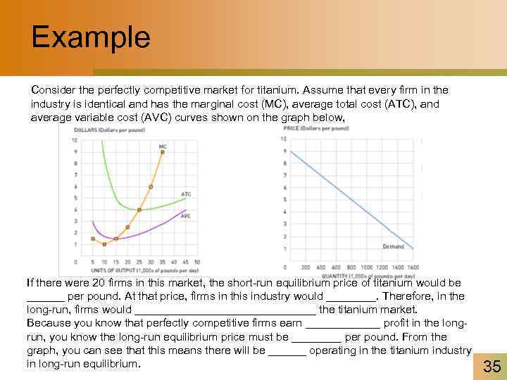Example Consider the perfectly competitive market for titanium. Assume that every firm in the industry is identical and has the marginal cost (MC), average total cost (ATC), and average variable cost (AVC) curves shown on the graph below, If there were 20 firms in this market, the short-run equilibrium price of titanium would be ______ per pound. At that price, firms in this industry would ____. Therefore, in the long-run, firms would _______________ the titanium market. Because you know that perfectly competitive firms earn ______ profit in the longrun, you know the long-run equilibrium price must be ____ per pound. From the graph, you can see that this means there will be ______ operating in the titanium industry in long-run equilibrium. 35

Changes in Plant Size • Firms change their plant size whenever doing so is profitable. • If average total cost exceeds the minimum long-run average cost, firms change their plant size to lower costs and increase profits. 36

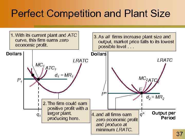Perfect Competition and Plant Size 1. With its current plant and ATC curve, this firm earns zero economic profit. Dollars MC 1 P 1 3. As all firms increase plant size and output, market price falls to its lowest possible level. . . LRATC ATC 1 d 1 = MR 1 MC 2 ATC P* 2 E 2. The firm could earn positive profit with a Output per 4. and all firms earn q 1 larger plant, q* Period producing here. zero. economic profit and produce at minimum LRATC. d 2 = MR 2 Output per Period 37

Long-Run Equilibrium Long-run equilibrium occurs in a competitive industry when: – Economic profit is zero, so firms neither enter nor exit the industry. – Long-run average cost is at its minimum, so firms don’t change their plant size. 38

A Change in Demand • Short-run impact of an increase in demand is – Rise in market price – Rise in market quantity – Economic profits • Long-run supply curve – Curve indicating quantity of output that all sellers in a market will produce at different prices After all long-run adjustments have taken place 39

Increasing, Decreasing, and Constant Cost Industries • Increase in demand for inputs causes price of those inputs to rise • This type of industry (which is the most common) is called an increasing cost industry – Entry causes input prices to rise • Shifts typical firm’s ATC curve up – Raises market price at which firms earn zero economic profit » As a result, long-run supply curve slopes upward 40

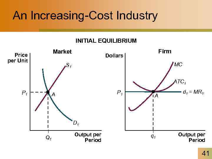An Increasing-Cost Industry INITIAL EQUILIBRIUM Market Price per Unit Firm Dollars MC S 1 ATC 1 P 1 A A d 1 = MR 1 D 1 Q 1 Output per Period q 1 Output per Period 41

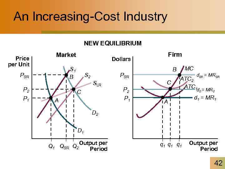An Increasing-Cost Industry NEW EQUILIBRIUM Price per Unit Market S 1 B PSR P 1 S 2 C C P 2 P 1 A MC B PSR SLR P 2 Firm Dollars d = MRSR ATC 2 SR ATC 1 d = MR 2 A 2 d 1 = MR 1 D 2 D 1 QSR Q 2 Output per Period q 1 q 1 Output per Period 42

Increasing, Decreasing, and Constant Cost Industries • Industry might use such a small percentage of total inputs that—even as new firms enter—there is no noticeable effect on input prices: a constant cost industry • Entry has no effect on input prices, so typical firm’s ATC curve stays put – Long-run supply curve is horizontal • Decreasing cost industry, in which entry by new firms actually decreases input prices – Causes typical firm’s ATC curve to shift downward – Lowers market price at which firms earn zero economic profit – As a result, long-run supply curve slopes downward 43

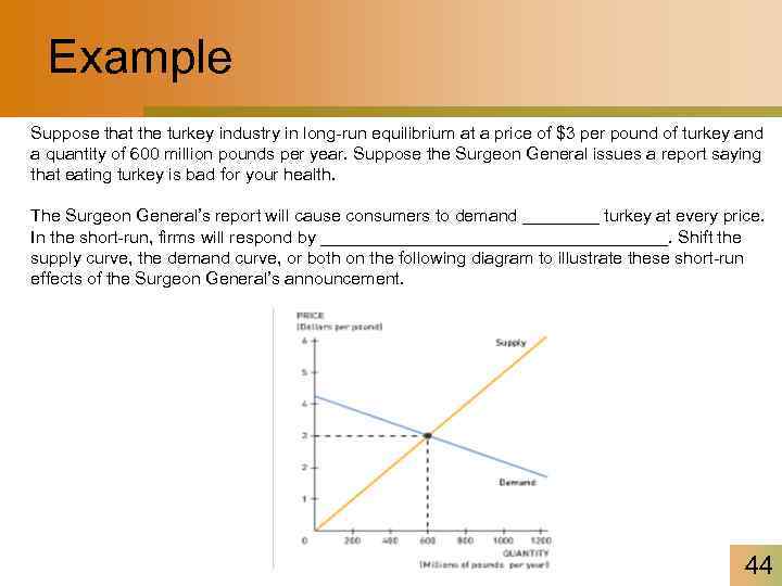Example Suppose that the turkey industry in long-run equilibrium at a price of $3 per pound of turkey and a quantity of 600 million pounds per year. Suppose the Surgeon General issues a report saying that eating turkey is bad for your health. The Surgeon General’s report will cause consumers to demand ____ turkey at every price. In the short-run, firms will respond by __________________. Shift the supply curve, the demand curve, or both on the following diagram to illustrate these short-run effects of the Surgeon General’s announcement. 44

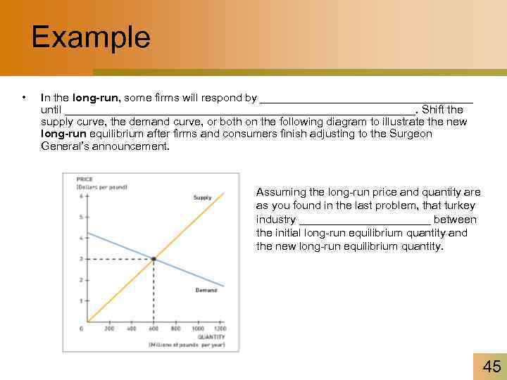Example • In the long-run, some firms will respond by _________________ until ____________________________. Shift the supply curve, the demand curve, or both on the following diagram to illustrate the new long-run equilibrium after firms and consumers finish adjusting to the Surgeon General’s announcement. Assuming the long-run price and quantity are as you found in the last problem, that turkey industry ___________ between the initial long-run equilibrium quantity and the new long-run equilibrium quantity. 45

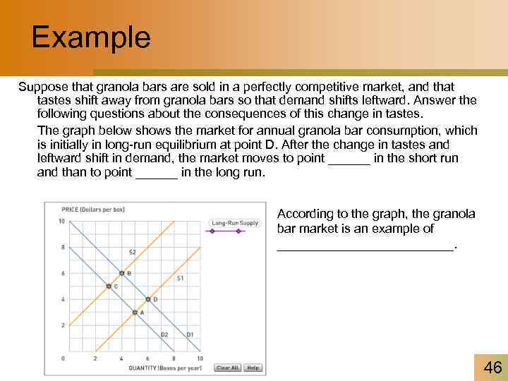Example Suppose that granola bars are sold in a perfectly competitive market, and that tastes shift away from granola bars so that demand shifts leftward. Answer the following questions about the consequences of this change in tastes. The graph below shows the market for annual granola bar consumption, which is initially in long-run equilibrium at point D. After the change in tastes and leftward shift in demand, the market moves to point ______ in the short run and than to point ______ in the long run. According to the graph, the granola bar market is an example of _____________. 46

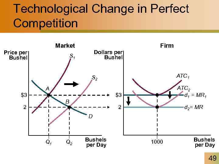
Advancing Technology • Technological Change – New technologies are constantly discovered that lower costs. – A new technology enables firms to producer at a lower average cost and lower marginal cost—firms’ cost curves shift downward. – Firms that adopt the new technology earn an economic profit. 47

Changing Tastes and Advancing Technology – New-technology firms enter and old-technology firms either exit or adopt the new technology. – Industry supply increases and the industry supply curve shifts rightward. – The price falls and the quantity increases. – Eventually, a new long-run equilibrium emerges in which all the firms use the new technology, the price has fallen to the minimum average total cost, and each firm earns normal profit. 48

Technological Change in Perfect Competition Firm Market Price per Bushel Dollars per Bushel S 1 ATC 1 S 2 ATC 2 d 1 = MR 1 A $3 $3 B 2 d 2= MR 2 D Q 1 Q 2 Bushels per Day 1000 Bushels per Day 49

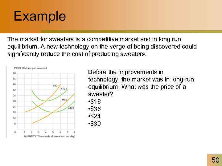Example The market for sweaters is a competitive market and in long run equilibrium. A new technology on the verge of being discovered could significantly reduce the cost of producing sweaters. Before the improvements in technology, the market was in long-run equilibrium. What was the price of a sweater? • $18 • $36 • $24 • $30 50

Example • • Suppose one firm discovers the new technology and is the only able to use it. Approximately how much profit would that firm make? (You can safety assume that one firm’s production decisions do not affect the market price. ) $210, 000 per day Zero additional profit $24, 000 per day $42, 000 per day Assume that all existing firms in this industry adopt the new cost-cutting technology and begin earning profit. In the long run, the profit generated by technological improvement will cause firms to _____ the industry until the long-run price of a sweater equals _____. 51