Comparison of Pooled and Household -Level Usage Impact

Comparison of Pooled and Household -Level Usage Impact Analysis Jackie Berger Ferit Ucar IEPEC Conference – August 14, 2013

Presentation Outline • • • Motivation Billing Analysis Usage Impact Models Model Results Summary and Next Steps 2

MOTIVATION 3

Usage Impacts • • • Were expected energy savings results obtained? Are the treatments cost-effective? Should measure selection procedures be revised? Should installation procedures be reviewed? Should contractors be re-trained? 4

Analysis Method • Goal: develop most accurate estimate of program savings. • Weigh costs and benefits of various approaches to measurement. • Consider possible causes of mis-measurement or bias. 5

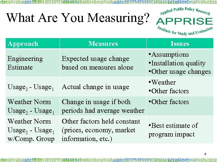What Are You Measuring? Approach Engineering Estimate Measures Expected usage change based on measures alone Issues • Assumptions • Installation quality • Other usage changes • Weather • Other factors Usage 2 - Usage 1 Actual change in usage Weather Norm Usage 2 - Usage 1 w/Comp. Group Change in usage if both periods had average weather Other factors held constant • Best estimate of (prices, economy, market program impact information, etc. ) 6

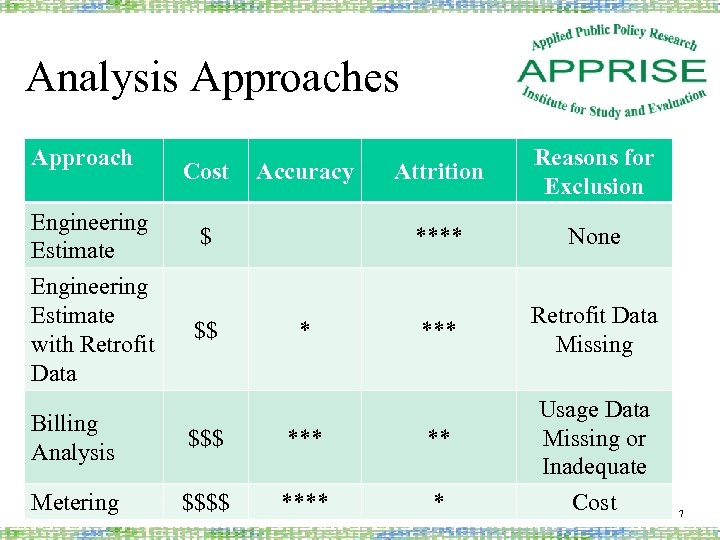Analysis Approaches Approach Engineering Estimate with Retrofit Data Cost $ $$ * Attrition Reasons for Exclusion **** Accuracy None *** Retrofit Data Missing Billing Analysis $$$ *** ** Metering $$$$ **** * Usage Data Missing or Inadequate Cost 7

Billing Analysis 8

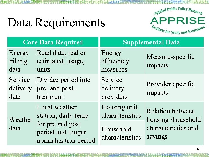Data Requirements Core Data Required Energy Read date, real or billing estimated, usage, data units Supplemental Data Energy Measure-specific efficiency impacts measures Service Divides period into delivery pre- and postdate treatment Service delivery providers Local weather station, daily temp Weather for pre and post data period and longer normalization period Housing unit Relation between characteristics housing /household characteristics and Household characteristics savings Provider-specific impacts 9

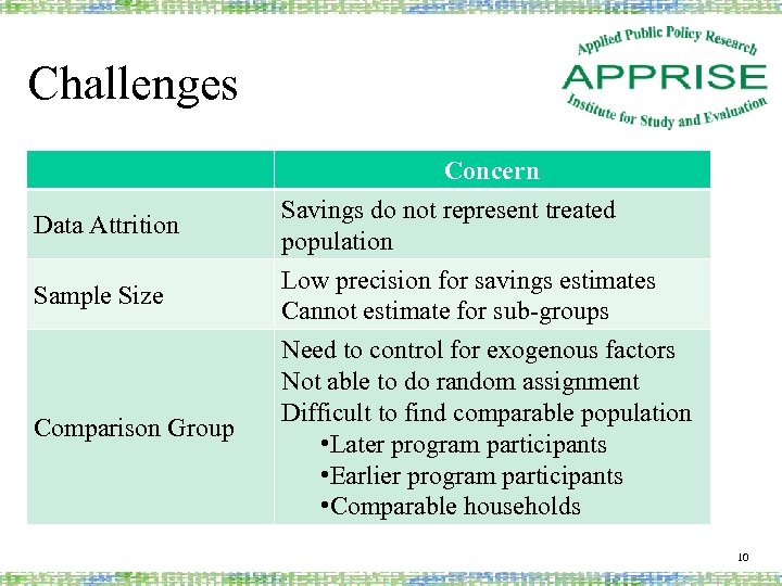Challenges Data Attrition Concern Savings do not represent treated population Sample Size Low precision for savings estimates Cannot estimate for sub-groups Comparison Group Need to control for exogenous factors Not able to do random assignment Difficult to find comparable population • Later program participants • Earlier program participants • Comparable households 10

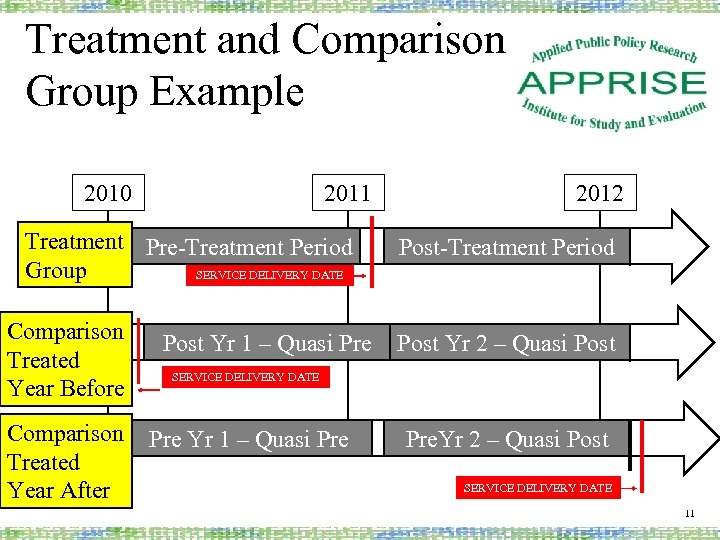Treatment and Comparison Group Example 2010 2011 Treatment Pre-Treatment Period Group SERVICE DELIVERY DATE Comparison Treated Year Before Comparison Treated Year After Post Yr 1 – Quasi Pre 2012 Post-Treatment Period Post Yr 2 – Quasi Post SERVICE DELIVERY DATE Pre Yr 1 – Quasi Pre. Yr 2 – Quasi Post SERVICE DELIVERY DATE 11

Usage Impact Models 12

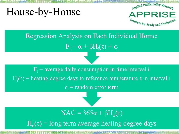House-by-House Regression Analysis on Each Individual Home: Fi = α + βHi(τ) + ϵi Fi = average daily consumption in time interval i Hi(τ) = heating degree days to reference temperature τ in interval i ϵi = random error term NAC = 365α + βHo(τ) Ho(τ) = long term average heating degree days 13

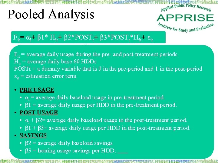Pooled Analysis Fit= αi+ β 1* Hit+ β 2*POSTt+ β 3*POSTt*Hit+ εit Fit = average daily usage during the pre- and post-treatment periods Hit = average daily base 60 HDDs POSTt = a dummy variable that is 0 in the pre-period and 1 in the post-period εit = estimation error term • PRE USAGE • αi = average daily baseload usage in pre-treatment period. • β 1 = average daily usage per HDD in the pre-treatment period. • POST USAGE • αi + β 2= average daily baseload usage in the post-treatment period. • β 1 + β 3= average daily usage per HDD in the post-treatment period. • SAVINGS • β 2 = average daily baseload savings • β 3 = heating usage savings per HDD. 14

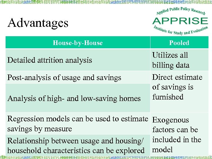Advantages House-by-House Detailed attrition analysis Post-analysis of usage and savings Analysis of high- and low-saving homes Pooled Utilizes all billing data Direct estimate of savings is furnished Regression models can be used to estimate Exogenous savings by measure factors can be Relationship between usage and housing/ included in the household characteristics can be explored model 15

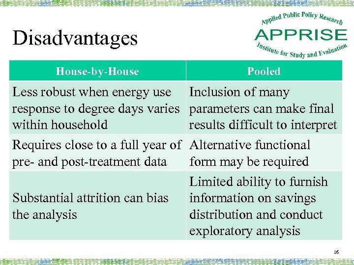Disadvantages House-by-House Pooled Less robust when energy use response to degree days varies within household Requires close to a full year of pre- and post-treatment data Inclusion of many parameters can make final results difficult to interpret Alternative functional form may be required Limited ability to furnish information on savings distribution and conduct exploratory analysis Substantial attrition can bias the analysis 16

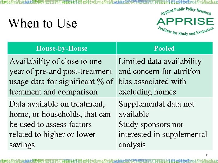When to Use House-by-House Pooled Availability of close to one year of pre-and post-treatment usage data for significant % of treatment and comparison Data available on treatment, home, or households, that can be used to assess factors related to higher or lower savings Limited data availability and concern for attrition bias associated with excluding homes Supplemental data not available Study sponsors not interested in supplemental analysis 17

Model Results 18

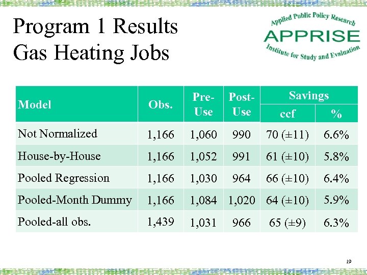Program 1 Results Gas Heating Jobs Post. Use Savings ccf % Model Obs. Pre. Use Not Normalized 1, 166 1, 060 990 70 (± 11) 6. 6% House-by-House 1, 166 1, 052 991 61 (± 10) 5. 8% Pooled Regression 1, 166 1, 030 964 66 (± 10) 6. 4% Pooled-Month Dummy 1, 166 1, 084 1, 020 64 (± 10) 5. 9% Pooled-all obs. 1, 439 1, 031 6. 3% 966 65 (± 9) 19

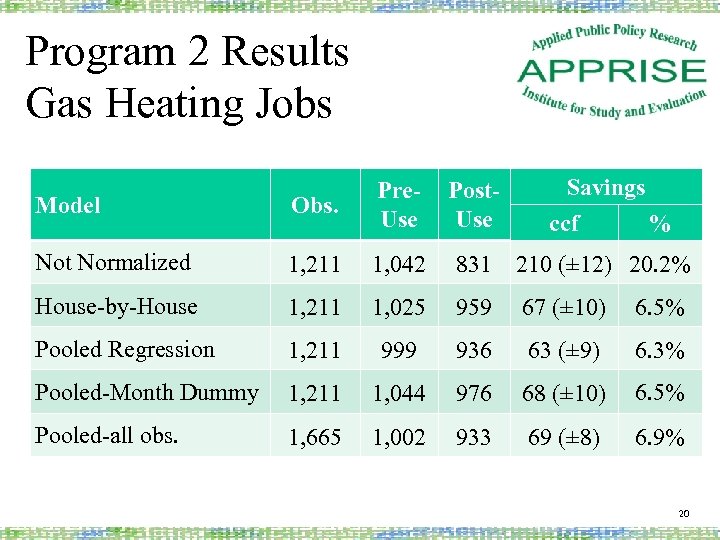Program 2 Results Gas Heating Jobs Post. Use Savings ccf % Model Obs. Pre. Use Not Normalized 1, 211 1, 042 831 210 (± 12) 20. 2% House-by-House 1, 211 1, 025 959 67 (± 10) 6. 5% Pooled Regression 1, 211 999 936 63 (± 9) 6. 3% Pooled-Month Dummy 1, 211 1, 044 976 68 (± 10) 6. 5% Pooled-all obs. 1, 665 1, 002 933 69 (± 8) 6. 9% 20

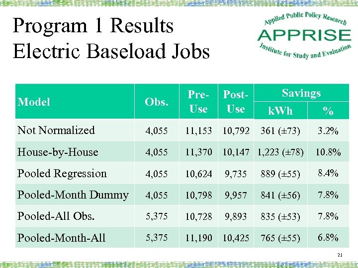Program 1 Results Electric Baseload Jobs Post. Use Savings k. Wh % Model Obs. Pre. Use Not Normalized 4, 055 11, 153 10, 792 House-by-House 4, 055 11, 370 10, 147 1, 223 (± 78) 10. 8% Pooled Regression 4, 055 10, 624 9, 735 889 (± 55) 8. 4% Pooled-Month Dummy 4, 055 10, 798 9, 957 841 (± 56) 7. 8% Pooled-All Obs. 5, 375 10, 728 9, 893 835 (± 53) 7. 8% Pooled-Month-All 5, 375 11, 190 10, 425 765 (± 55) 6. 8% 361 (± 73) 3. 2% 21

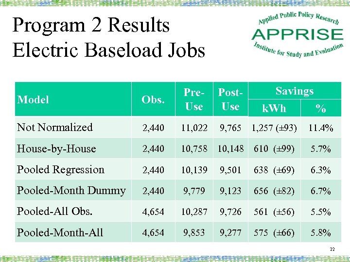Program 2 Results Electric Baseload Jobs Post. Use Savings k. Wh % Model Obs. Pre. Use Not Normalized 2, 440 11, 022 9, 765 1, 257 (± 93) 11. 4% House-by-House 2, 440 10, 758 10, 148 610 (± 99) 5. 7% Pooled Regression 2, 440 10, 139 9, 501 638 (± 69) 6. 3% Pooled-Month Dummy 2, 440 9, 779 9, 123 656 (± 82) 6. 7% Pooled-All Obs. 4, 654 10, 287 9, 726 561 (± 56) 5. 5% Pooled-Month-All 4, 654 9, 853 9, 277 575 (± 66) 5. 8% 22

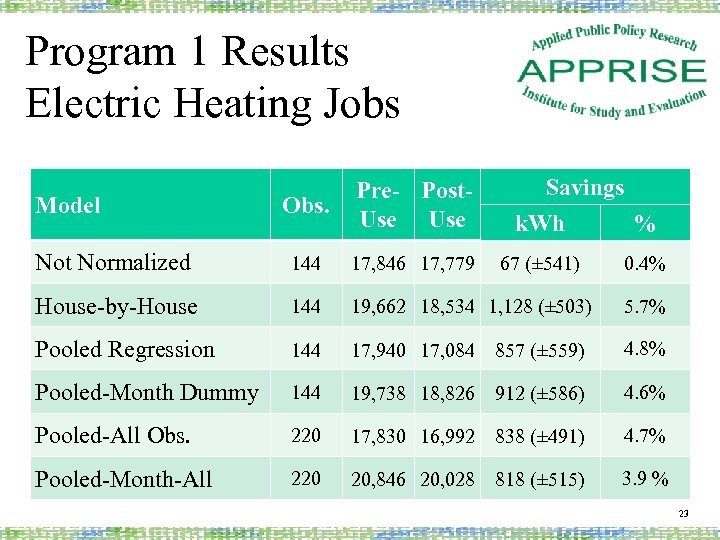Program 1 Results Electric Heating Jobs Savings k. Wh % Obs. Pre- Post. Use Not Normalized 144 17, 846 17, 779 House-by-House 144 19, 662 18, 534 1, 128 (± 503) 5. 7% Pooled Regression 144 17, 940 17, 084 857 (± 559) 4. 8% Pooled-Month Dummy 144 19, 738 18, 826 912 (± 586) 4. 6% Pooled-All Obs. 220 17, 830 16, 992 838 (± 491) 4. 7% Pooled-Month-All 220 20, 846 20, 028 818 (± 515) 3. 9 % Model 67 (± 541) 0. 4% 23

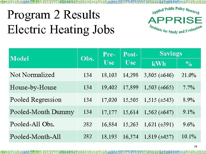Program 2 Results Electric Heating Jobs Savings k. Wh % Obs. Pre. Use Post. Use Not Normalized 134 18, 103 14, 298 3, 805 (± 646) 21. 0% House-by-House 134 19, 402 17, 899 1, 503 (± 665) 7. 7% Pooled Regression 134 17, 020 15, 505 1, 515 (± 543) 8. 9% Pooled-Month Dummy 134 17, 177 15, 614 1, 562 (± 647) 9. 1% Pooled-All Obs. 282 16, 884 15, 263 1, 621 (± 391) 9. 6% Pooled-Month-All 282 18, 193 16, 374 1, 819 (± 457) 10. 1% Model 24

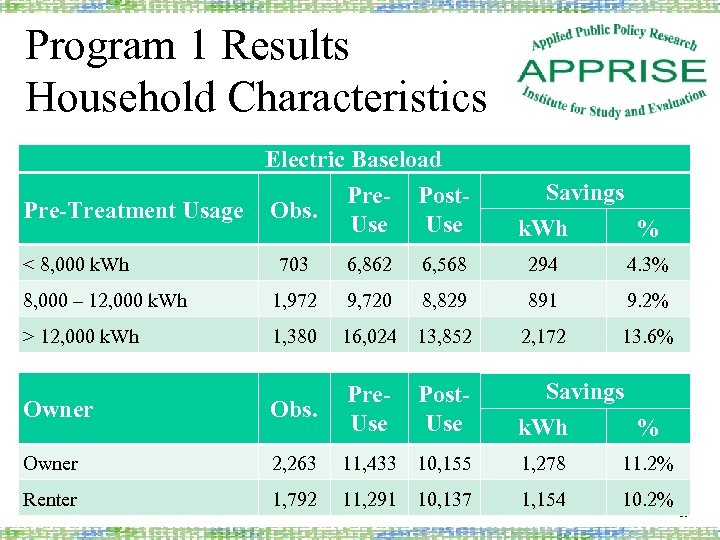Program 1 Results Household Characteristics Electric Baseload Pre- Post. Pre-Treatment Usage Obs. Use < 8, 000 k. Wh Savings k. Wh % 703 6, 862 6, 568 294 4. 3% 8, 000 – 12, 000 k. Wh 1, 972 9, 720 8, 829 891 9. 2% > 12, 000 k. Wh 1, 380 16, 024 13, 852 2, 172 13. 6% Owner Obs. Pre. Use Post. Use Savings k. Wh % Owner 2, 263 11, 433 10, 155 1, 278 11. 2% Renter 1, 792 11, 291 10, 137 1, 154 10. 2% 25

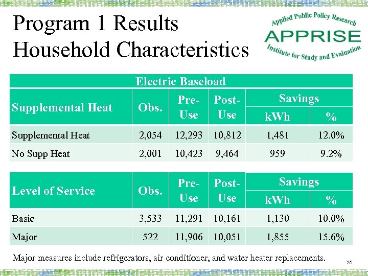Program 1 Results Household Characteristics Supplemental Heat Electric Baseload Pre- Post. Obs. Use Savings k. Wh % Supplemental Heat 2, 054 12, 293 10, 812 1, 481 12. 0% No Supp Heat 2, 001 10, 423 9, 464 959 9. 2% Level of Service Obs. Pre. Use Post. Use Savings k. Wh % Basic 3, 533 11, 291 10, 161 1, 130 10. 0% Major 522 11, 906 10, 051 1, 855 15. 6% Major measures include refrigerators, air conditioner, and water heater replacements. 26

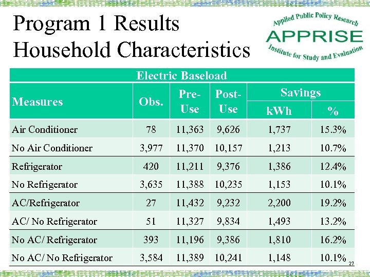Program 1 Results Household Characteristics Measures Air Conditioner Electric Baseload Pre- Post. Obs. Use Savings k. Wh % 78 11, 363 9, 626 1, 737 15. 3% 3, 977 11, 370 10, 157 1, 213 10. 7% 420 11, 211 9, 376 1, 386 12. 4% No Refrigerator 3, 635 11, 388 10, 235 1, 153 10. 1% AC/Refrigerator 27 11, 432 9, 232 2, 200 19. 2% AC/ No Refrigerator 51 11, 327 9, 834 1, 493 13. 2% No AC/ Refrigerator 393 11, 196 9, 386 1, 810 16. 2% 3, 584 11, 389 10, 241 1, 148 10. 1% 27 No Air Conditioner Refrigerator No AC/ No Refrigerator

Summary and Next Steps 28

Summary • Overall savings results fairly consistent • Differences between models rarely statistically significant • Gas usage results were more consistent • Electric baseload varied most 29

Conclusions • Sources and potential biases caused by large data attrition should be explored. • When additional analysis is desired for many subgroups and data attrition is low, house-byhouse may be favored. • When data attrition is high and only overall usage results are desired, the pooled regression may be preferred. 30

Next Steps • Additional exploration of differences. • Explore deletion of various types and numbers of observations from house by house. • Compare results with different levels of attrition. • Test different functional forms for the pooled model. 31