COMP 9517 Computer Vision Motion 3 17 2018 COMP 9517

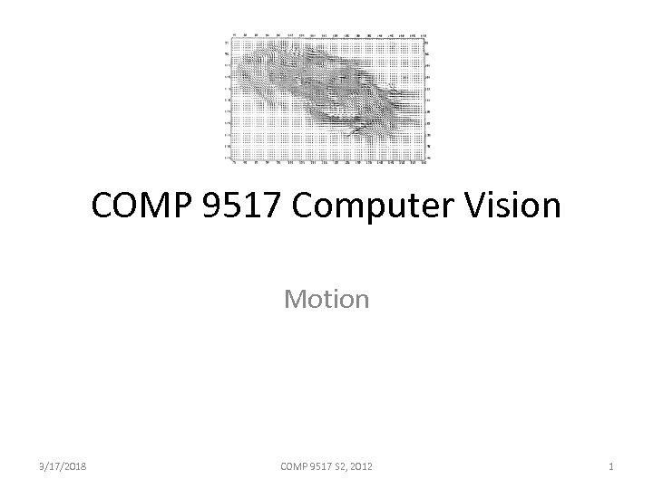COMP 9517 Computer Vision Motion 3/17/2018 COMP 9517 S 2, 2012 1

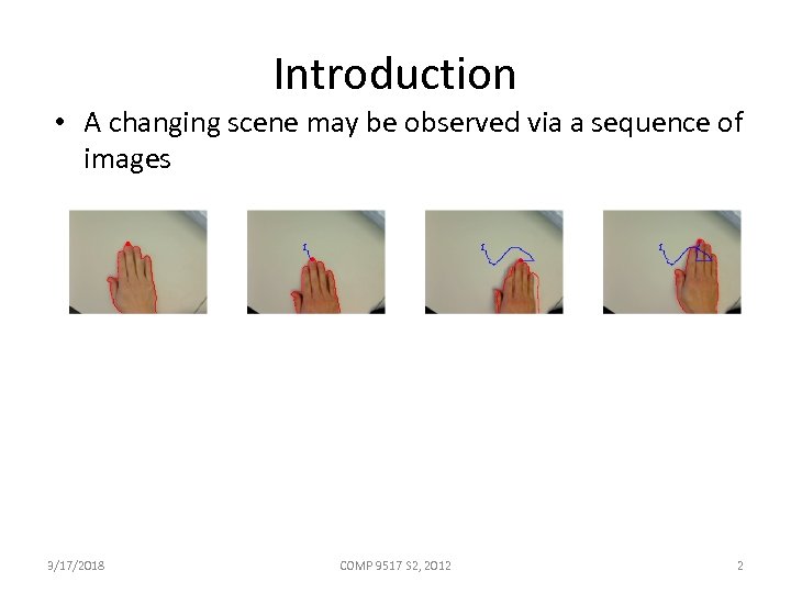Introduction • A changing scene may be observed via a sequence of images 3/17/2018 COMP 9517 S 2, 2012 2

Introduction • Changes in an image sequence provide features for – – – 3/17/2018 detecting objects that are moving computing their trajectories computing the motion of the viewer in the world recognising objects based on their behaviours detecting and recognising activities COMP 9517 S 2, 2012 3

Applications • Motion-based recognition: human identification based on gait, automatic object detection, etc; • Automated surveillance: monitoring a scene to detect suspicious activities or unlikely events; • Video indexing: automatic annotation and retrieval of the videos in multimedia databases; • Human-computer interaction: gesture recognition, eye gaze tracking for data input to computers, etc. ; • Traffic monitoring: real-time gathering of traffic statistics to direct traffic flow. • Vehicle navigation: video-based path planning and obstacle avoidance capabilities. 3/17/2018 COMP 9517 S 2, 2012 4

Motion Phenomena 1) Still camera, single moving object, constant background 2) Still camera, several moving objects, constant background 3) Moving camera, relatively constant scene 4) Moving camera, several moving objects 3/17/2018 COMP 9517 S 2, 2012 5

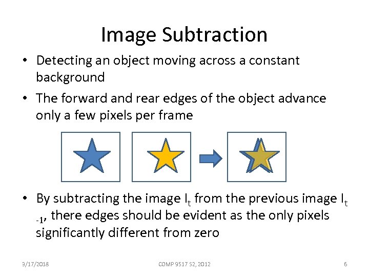Image Subtraction • Detecting an object moving across a constant background • The forward and rear edges of the object advance only a few pixels per frame • By subtracting the image It from the previous image It -1, there edges should be evident as the only pixels significantly different from zero 3/17/2018 COMP 9517 S 2, 2012 6

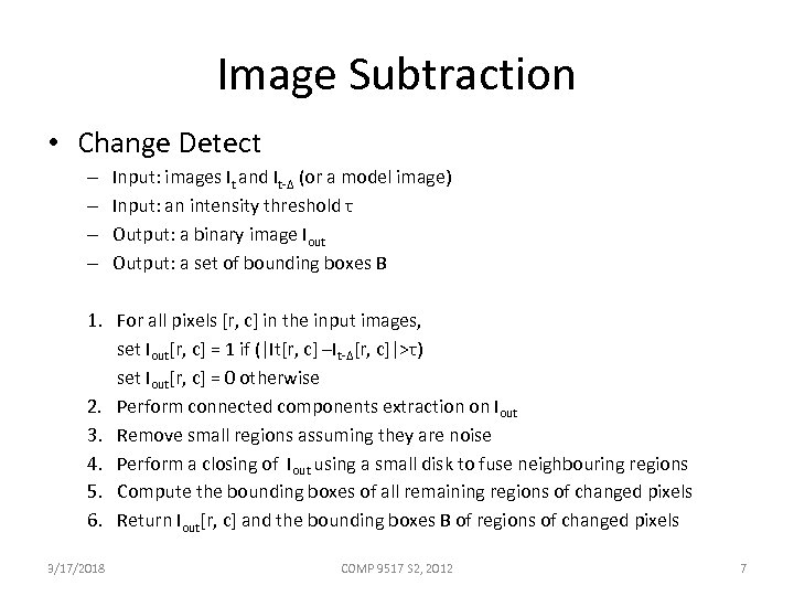Image Subtraction • Change Detect – – Input: images It and It-Δ (or a model image) Input: an intensity threshold τ Output: a binary image Iout Output: a set of bounding boxes B 1. For all pixels [r, c] in the input images, set Iout[r, c] = 1 if (|It[r, c] –It-Δ[r, c]|>τ) set Iout[r, c] = 0 otherwise 2. Perform connected components extraction on Iout 3. Remove small regions assuming they are noise 4. Perform a closing of Iout using a small disk to fuse neighbouring regions 5. Compute the bounding boxes of all remaining regions of changed pixels 6. Return Iout[r, c] and the bounding boxes B of regions of changed pixels 3/17/2018 COMP 9517 S 2, 2012 7

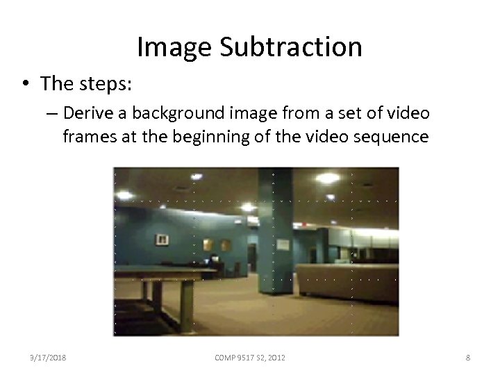Image Subtraction • The steps: – Derive a background image from a set of video frames at the beginning of the video sequence 3/17/2018 COMP 9517 S 2, 2012 8

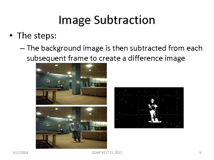Image Subtraction • The steps: – The background image is then subtracted from each subsequent frame to create a difference image 3/17/2018 COMP 9517 S 2, 2012 9

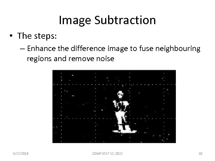Image Subtraction • The steps: – Enhance the difference image to fuse neighbouring regions and remove noise 3/17/2018 COMP 9517 S 2, 2012 10

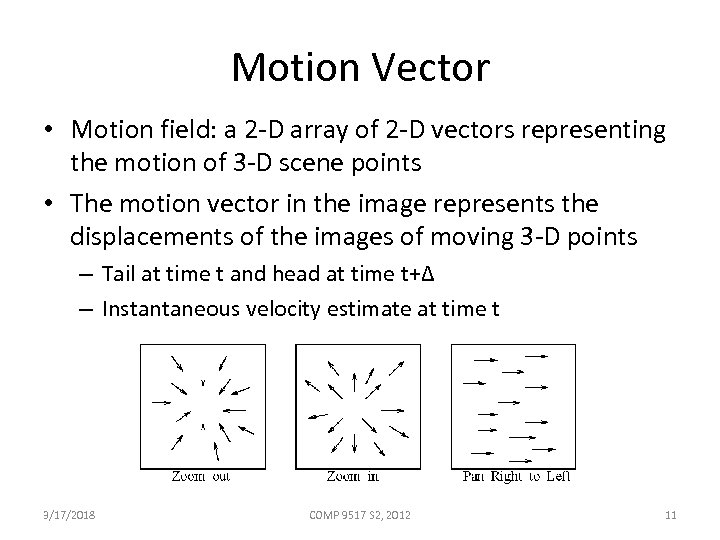Motion Vector • Motion field: a 2 -D array of 2 -D vectors representing the motion of 3 -D scene points • The motion vector in the image represents the displacements of the images of moving 3 -D points – Tail at time t and head at time t+Δ – Instantaneous velocity estimate at time t 3/17/2018 COMP 9517 S 2, 2012 11

Motion Vector • Two assumption: – The intensity of a 3 -D scene point and that of its neighbours remain nearly constant during the time interval – The intensity differences observed along the images of the edges of objects are nearly constant during the time interval • Image flow: the motion field computed under the assumption that image intensity near corresponding points is relatively constant • Two methods for computing image flow: – Sparse: point correspondence-based method – Dense: spatial & temporal gradient-based method 3/17/2018 COMP 9517 S 2, 2012 12

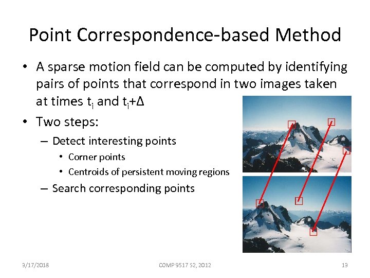Point Correspondence-based Method • A sparse motion field can be computed by identifying pairs of points that correspond in two images taken at times ti and ti+Δ • Two steps: – Detect interesting points • Corner points • Centroids of persistent moving regions – Search corresponding points 3/17/2018 COMP 9517 S 2, 2012 13

Point Correspondence-based Method • Detect interesting points: – Detect corner points • Kirsch edge operator • Frie-Chen ripple operator – Interest operator • Computes intensity variance in the vertical, horizontal and diagonal directions • Interest point if the minimum of these four variances exceeds a threshold 3/17/2018 COMP 9517 S 2, 2012 14

Point Correspondence-based Method • Finding interesting points of a given input image Procedure detect_corner_points(I, V){ for (r = 0 to Max. Row – 1) for (c = 0 to Max. Col – 1) if (I[r, c] is a border pixel) break; elseif (interest_operator(I, r, c, w)>=t) add [(r, c), (r, c)] to set V; } Procedure interest_opertator (I, r, c, w){ v 1 = variance of intensity of horizontal pixels I[r, c-w]…I[r, c-w]; v 2 = variance of intensity of vertical pixels I[r-w, c]…I[r+w, ]; v 3 = variance of intensity of diagonal pixels I[r-w, c-w]…I[r+w, c+w]; v 4 = variance of intensity of diagonal pixels I[r-w, c+w]…I[r+w, c-w]; return mini(v 1, v 2, v 3, v 4); } 3/17/2018 COMP 9517 S 2, 2012 15

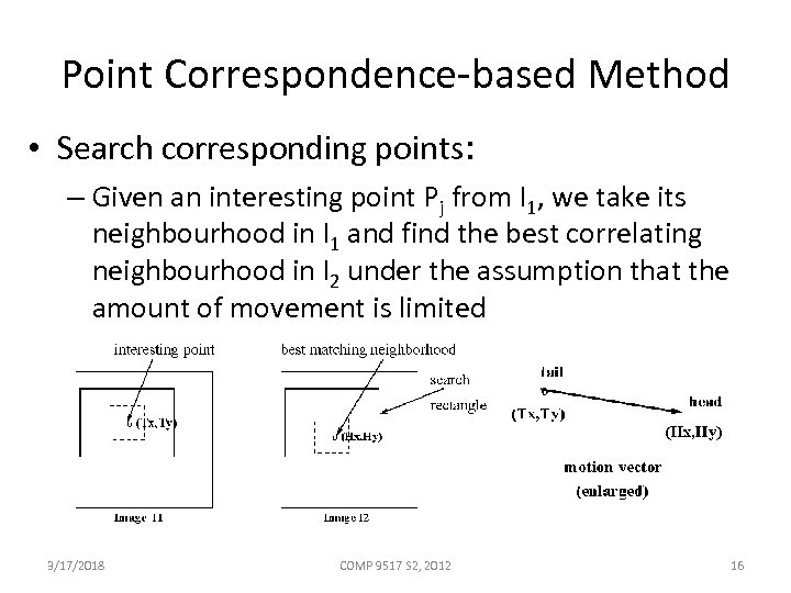Point Correspondence-based Method • Search corresponding points: – Given an interesting point Pj from I 1, we take its neighbourhood in I 1 and find the best correlating neighbourhood in I 2 under the assumption that the amount of movement is limited 3/17/2018 COMP 9517 S 2, 2012 16

Spatial & Temporal Gradient-based Method • Assumption – The object reflectivity and the illumination of the object do not change during the time interval – The distance of the object from the camera or light sources do not vary significantly over this interval – Each small intensity neighbourhood Nx, y at time t 1 is observed in some shifted position Nx+Δx, y+Δy at time t 2 • These assumption may be not hold tight in real case, but provides useful computation and approximation 3/17/2018 COMP 9517 S 2, 2012 17

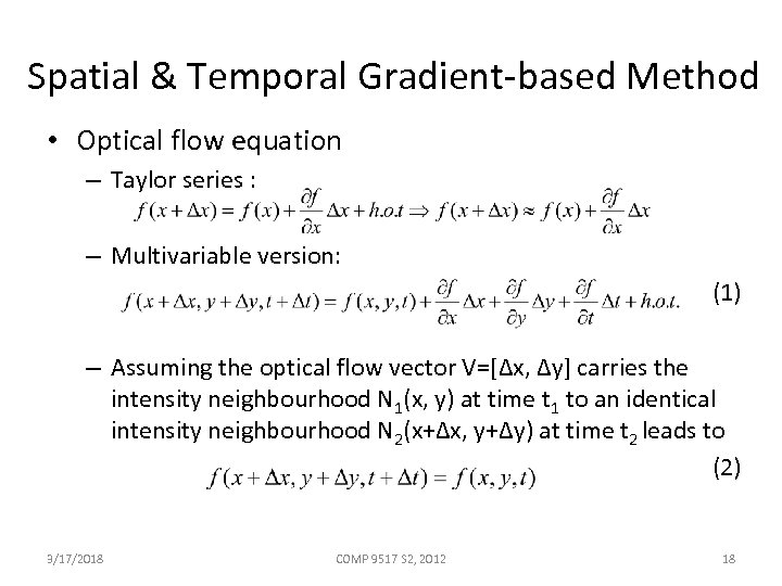Spatial & Temporal Gradient-based Method • Optical flow equation – Taylor series : – Multivariable version: (1) – Assuming the optical flow vector V=[Δx, Δy] carries the intensity neighbourhood N 1(x, y) at time t 1 to an identical intensity neighbourhood N 2(x+Δx, y+Δy) at time t 2 leads to (2) 3/17/2018 COMP 9517 S 2, 2012 18

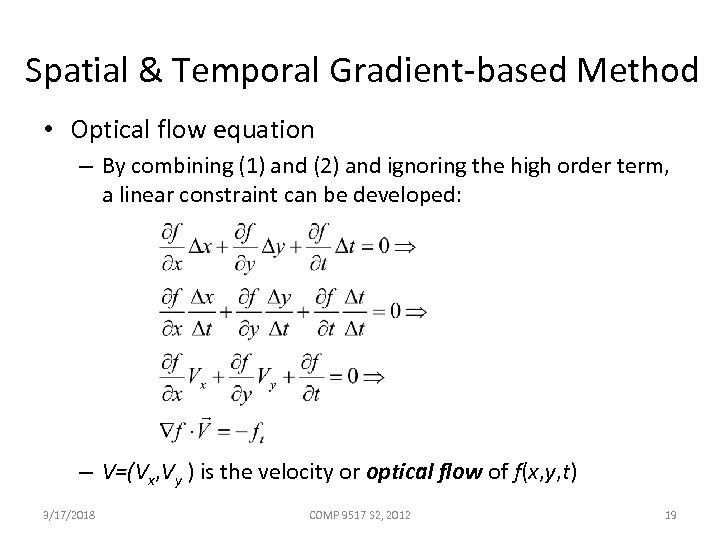Spatial & Temporal Gradient-based Method • Optical flow equation – By combining (1) and (2) and ignoring the high order term, a linear constraint can be developed: – V=(Vx, Vy ) is the velocity or optical flow of f(x, y, t) 3/17/2018 COMP 9517 S 2, 2012 19

Spatial & Temporal Gradient-based Method • The optical flow equation provides a constraint that can be applied at every pixel position • However, the optical flow does not give unique solution and thus further constrains are required – Example: using the optical flow equation for a group of adjacent pixels and assuming that all of them have the same velocity, the optical flow computation task is reduced to solving a linear system using the least square method 3/17/2018 COMP 9517 S 2, 2012 20

References and Acknowledgements • • 3/17/2018 Shapiro and Stockman 2001 Chapter 19 Forsyth and Ponce 2003 Chapter 5 Szeliski 2010 Images drawn from the above references unless otherwise mentioned COMP 9517 S 2, 2012 21