73668da924f248db9b12c5d2d860aa0f.ppt
- Количество слайдов: 67
COMP 9319 Web Data Compression and Search Revision
Course Aims As the amount of Web data increases, it is becoming vital to not only be able to search and retrieve this information quickly, but also to store it in a compact manner. This is especially important for mobile devices which are becoming increasingly popular. Without loss of generality, within this course, we assume Web data (excluding media content) will be in XML and its like (e. g. , XHTML). This course aims to introduce the concepts, theories, and algorithmic issues important to Web data compression and search. The course will also introduce the most recent development in various areas of Web data optimization topics, common practice, and its applications.
Assumed knowledge Official prerequisite of this course is COMP 2911/9024. At the start of this course students should be able to: • understand fundamental data structures. • produce correct programs in C/C++, i. e. , compilation, running, testing, debugging, etc. • produce readable code with clear documentation. • appreciate use of abstraction in computing.
Learning outcomes • have a good understanding of the fundamentals of text compression • be introduced to advanced data compression techniques such as those based on Burrows Wheeler Transform • have programming experience in Web data compression and optimization • have a deep understanding of XML and selected XML processing and optimization techniques • understand the advantages and disadvantages of data compression for Web search • have a basic understanding of XML distributed query processing • appreciate the past, present and future of data compression and Web data optimization
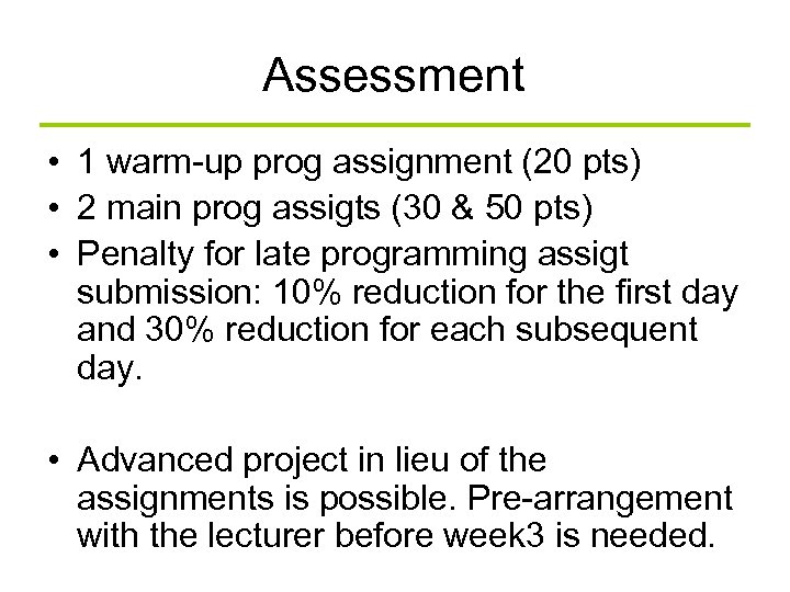
Assessment • 1 warm-up prog assignment (20 pts) • 2 main prog assigts (30 & 50 pts) • Penalty for late programming assigt submission: 10% reduction for the first day and 30% reduction for each subsequent day. • Advanced project in lieu of the assignments is possible. Pre-arrangement with the lecturer before week 3 is needed.
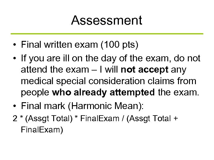
Assessment • Final written exam (100 pts) • If you are ill on the day of the exam, do not attend the exam – I will not accept any medical special consideration claims from people who already attempted the exam. • Final mark (Harmonic Mean): 2 * (Assgt Total) * Final. Exam / (Assgt Total + Final. Exam)
Assignments • Programming assignments are relatively challenging • In addition to correctness, specified performance parameters are required 7 7
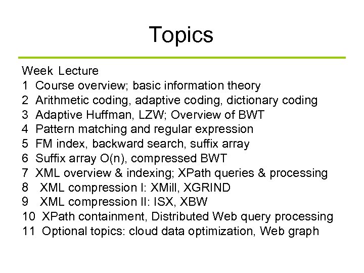
Topics Week Lecture 1 Course overview; basic information theory 2 Arithmetic coding, adaptive coding, dictionary coding 3 Adaptive Huffman, LZW; Overview of BWT 4 Pattern matching and regular expression 5 FM index, backward search, suffix array 6 Suffix array O(n), compressed BWT 7 XML overview & indexing; XPath queries & processing 8 XML compression I: XMill, XGRIND 9 XML compression II: ISX, XBW 10 XPath containment, Distributed Web query processing 11 Optional topics: cloud data optimization, Web graph
Final exam • 3 hours written exam • UNSW approved calculator – Remember to get the sticker before the exam • A single-sided A 4 sheet(typed or handwritten)
Exam preparation • Make sure you understand the slides (if needed, refer to the original papers) • Work on the exercises (before you check the answers) • Check and study the answers • Assignment related knowledge may be retested in the exam
Exam consultation • I’ll not be around in week 13 • Exam consultation during week 14 (study week): – In case you have question before the exam – Or you have question with the exercises – Or you have question with your assigt 3 score – Thurs 11: 00 -13: 00 – You can also post short questions to the msgboard
Yet to be done • Finish marking assignment 3 (you will receive results hopefully by end of wk 13) • For those assignment 2 with issues, you will receive your updated results in wk 13. • Follow up a few cases of potential plagiarism
Revision
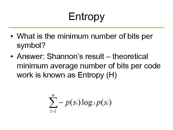
Entropy • What is the minimum number of bits per symbol? • Answer: Shannon’s result – theoretical minimum average number of bits per code work is known as Entropy (H)
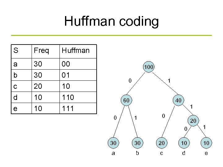
Huffman coding S Freq Huffman a b c 30 30 20 00 01 10 d e 10 10 111 100 0 1 60 40 1 0 20 0 1 30 30 20 10 10 a b c d e
Run-length coding • Run-length coding (encoding) is a very widely used and simple compression technique – does not assume a memoryless source – replace runs of symbols (possibly of length one) with pairs of (symbol, run-length)
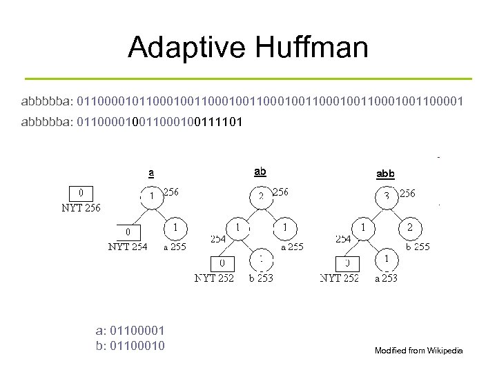
Adaptive Huffman abbbbba: 0110000101100010011000100110001001100001 abbbbba: 0110000100111101 a: 01100001 b: 01100010 Modified from Wikipedia
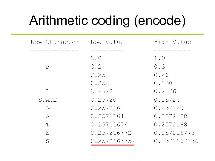
Arithmetic coding (encode)
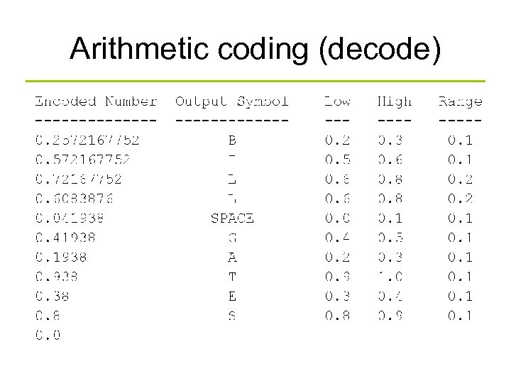
Arithmetic coding (decode)
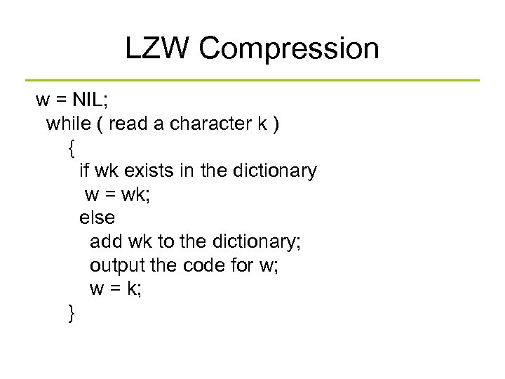
LZW Compression w = NIL; while ( read a character k ) { if wk exists in the dictionary w = wk; else add wk to the dictionary; output the code for w; w = k; }
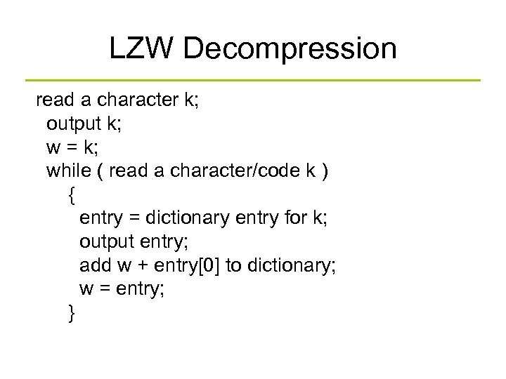
LZW Decompression read a character k; output k; w = k; while ( read a character/code k ) { entry = dictionary entry for k; output entry; add w + entry[0] to dictionary; w = entry; }
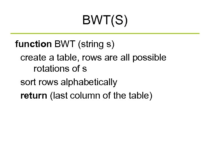
BWT(S) function BWT (string s) create a table, rows are all possible rotations of s sort rows alphabetically return (last column of the table)
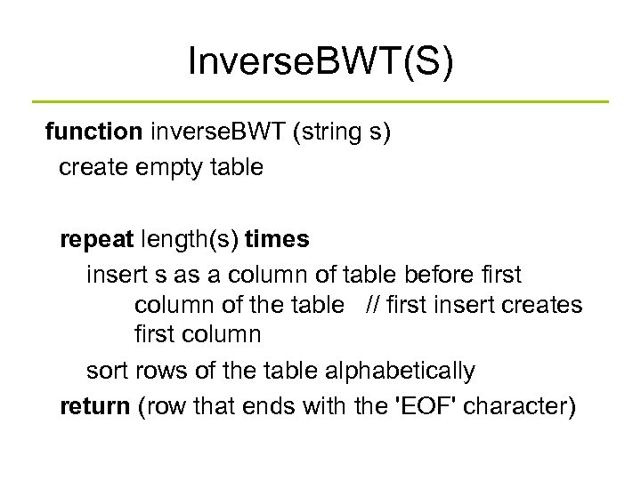
Inverse. BWT(S) function inverse. BWT (string s) create empty table repeat length(s) times insert s as a column of table before first column of the table // first insert creates first column sort rows of the table alphabetically return (row that ends with the 'EOF' character)
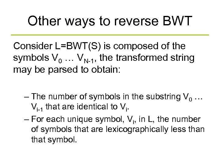
Other ways to reverse BWT Consider L=BWT(S) is composed of the symbols V 0 … VN-1, the transformed string may be parsed to obtain: – The number of symbols in the substring V 0 … Vi-1 that are identical to Vi. – For each unique symbol, Vi, in L, the number of symbols that are lexicographically less than that symbol.
Move to Front (MTF) • Reduce entropy based on local frequency correlation • Usually used for BWT before an entropyencoding step • Author and detail: – Original paper at cs 9319/Papers – http: //www. arturocampos. com/ac_mtf. html
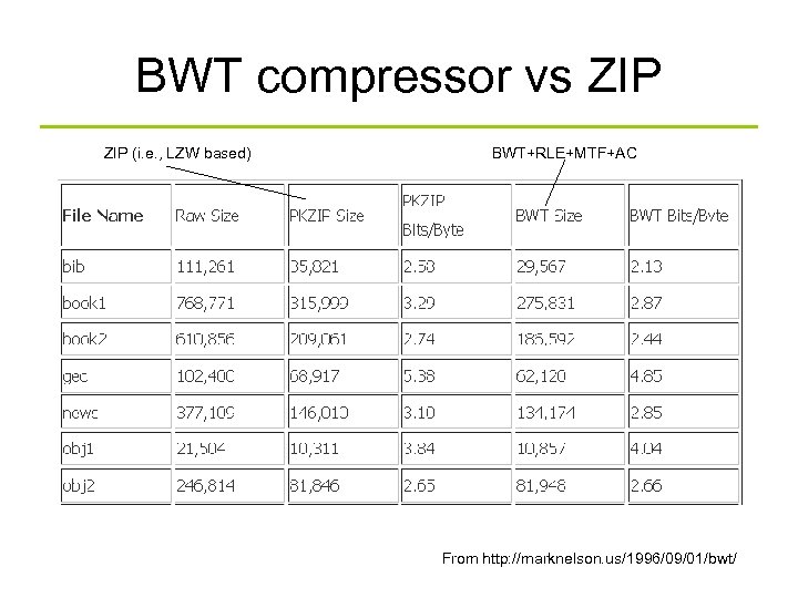
BWT compressor vs ZIP (i. e. , LZW based) BWT+RLE+MTF+AC From http: //marknelson. us/1996/09/01/bwt/
Pattern Matching • Definition: – given a text string T and a pattern string P, find the pattern inside the text • T: “the rain in spain stays mainly on the plain” • P: “n th”
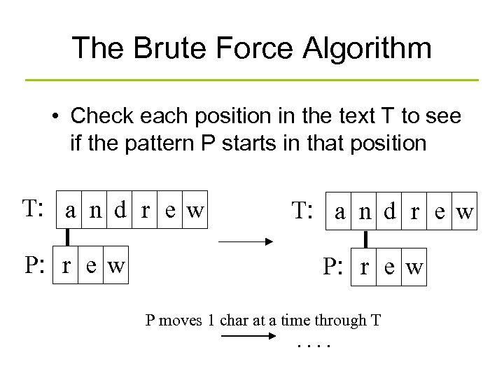
The Brute Force Algorithm • Check each position in the text T to see if the pattern P starts in that position T: a n d r e w P: r e w P moves 1 char at a time through T . .
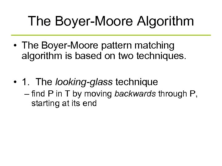
The Boyer-Moore Algorithm • The Boyer-Moore pattern matching algorithm is based on two techniques. • 1. The looking-glass technique – find P in T by moving backwards through P, starting at its end
![• 2. The character-jump technique – when a mismatch occurs at T[i] == • 2. The character-jump technique – when a mismatch occurs at T[i] ==](https://present5.com/presentation/73668da924f248db9b12c5d2d860aa0f/image-30.jpg)
• 2. The character-jump technique – when a mismatch occurs at T[i] == x – the character in pattern P[j] is not the same as T[i] • There are 3 possible cases. T P x a i ba j
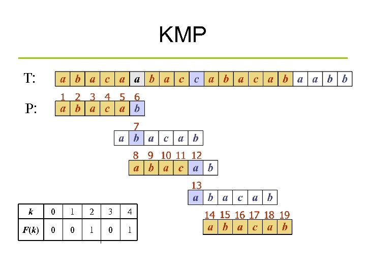
KMP T: P: k 0 1 2 3 4 F(k) 0 0 1
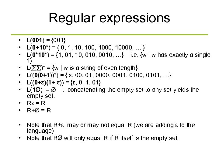
Regular expressions • L(001) = {001} • L(0+10*) = { 0, 1, 100, 10000, … } • L(0*10*) = {1, 01, 10, 0010, …} i. e. {w | w has exactly a single 1} • L( )* = {w | w is a string of even length} • L((0(0+1))*) = { ε, 00, 01, 0000, 0001, 0100, 0101, …} • L((0+ε)(1+ ε)) = {ε, 0, 1, 01} • L(1Ø) = Ø ; concatenating the empty set to any set yields the empty set. • Rε = R • R+Ø = R • Note that R+ε may or may not equal R (we are adding ε to the language) • Note that RØ will only equal R if R itself is the empty set.
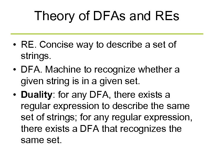
Theory of DFAs and REs • RE. Concise way to describe a set of strings. • DFA. Machine to recognize whether a given string is in a given set. • Duality: for any DFA, there exists a regular expression to describe the same set of strings; for any regular expression, there exists a DFA that recognizes the same set.
DFA to RE: State Elimination • Eliminates states of the automaton and replaces the edges with regular expressions that includes the behavior of the eliminated states. • Eventually we get down to the situation with just a start and final node, and this is easy to express as a RE
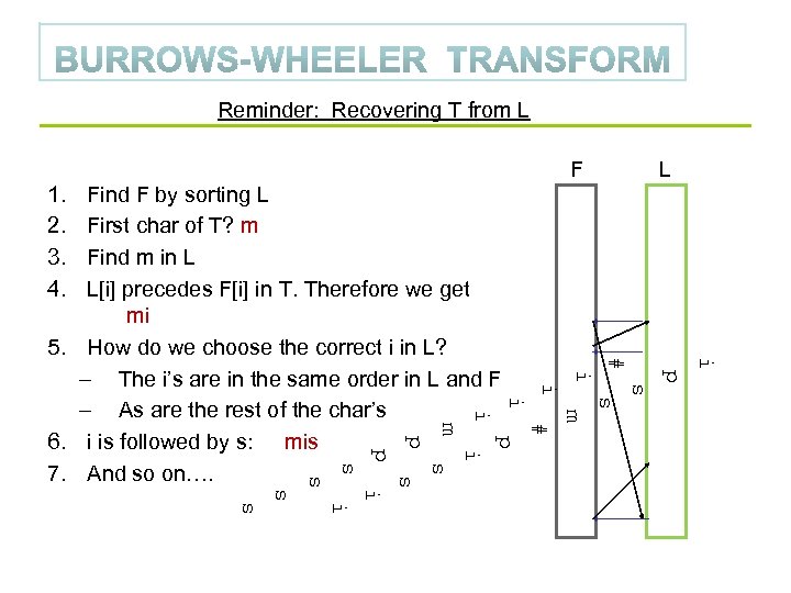
Reminder: Recovering T from L F L 1. 2. 3. 4. i # p i s i m i Find F by sorting L First char of T? m Find m in L L[i] precedes F[i] in T. Therefore we get mi 5. How do we choose the correct i in L? – The i’s are in the same order in L and F – As are the rest of the char’s 6. i is followed by s: mis 7. And so on…. # m p p i p s s i s
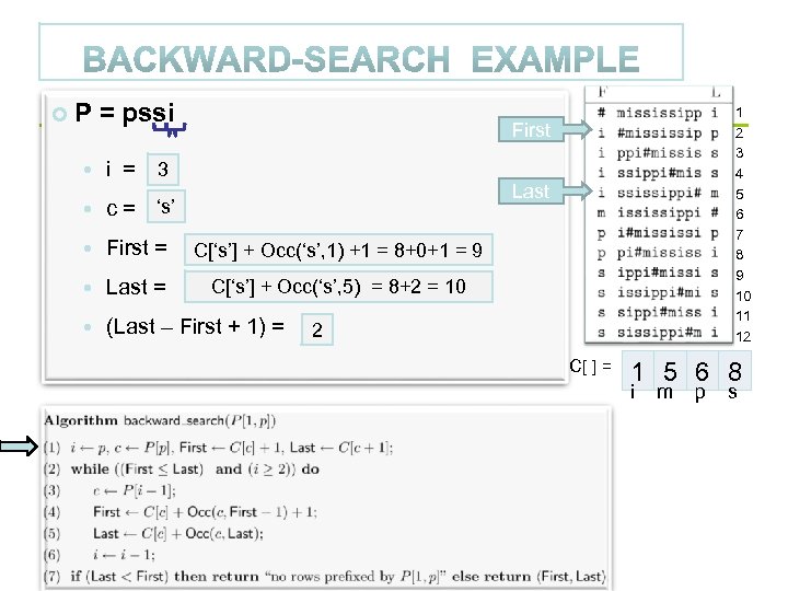
P = pssi 1 2 3 4 5 6 7 8 9 10 11 12 First 3 i = 4 Last ‘i’ ‘s’ c= First = C[‘s’] + Occ(‘s’, 1) +1 = 8+0+1 = 9 C[‘i’] + 1 = 2 Last = C[‘i’ + 1] Occ(‘s’, 5) 5 8+2 = 10 C[‘s’] + = C[‘m’] = = (Last – First + 1) = 2 4 C[ ] = 1 5 6 8 i m p s
Compression for inverted index § First, we will consider space for dictionary § Main motivation for dictionary compression: make it small enough to keep in main memory § Then for the postings file § Motivation: reduce disk space needed, decrease time needed to read from disk § Note: Large search engines keep significant part of postings in memory § We will devise various compression schemes for dictionary and postings. § VB code, Gamma code 37 37
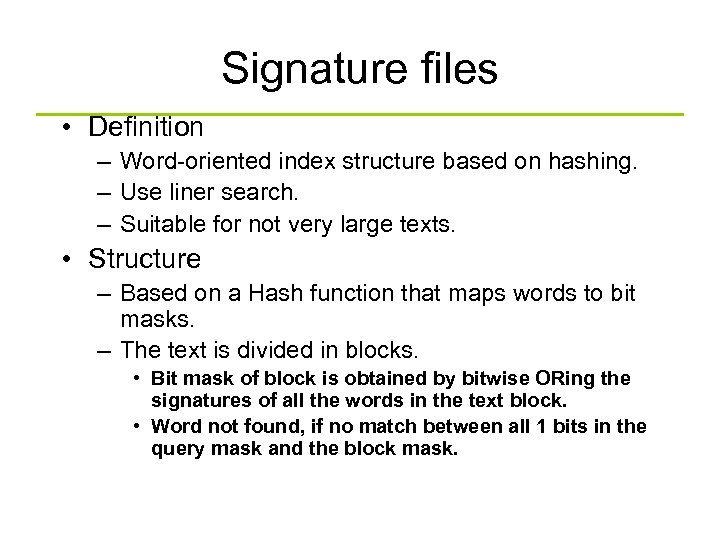
Signature files • Definition – Word-oriented index structure based on hashing. – Use liner search. – Suitable for not very large texts. • Structure – Based on a Hash function that maps words to bit masks. – The text is divided in blocks. • Bit mask of block is obtained by bitwise ORing the signatures of all the words in the text block. • Word not found, if no match between all 1 bits in the query mask and the block mask.
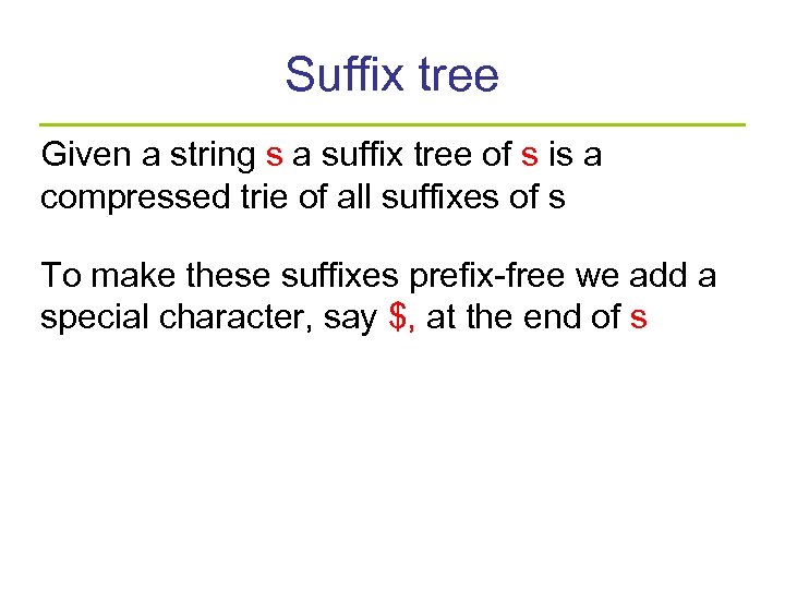
Suffix tree Given a string s a suffix tree of s is a compressed trie of all suffixes of s To make these suffixes prefix-free we add a special character, say $, at the end of s
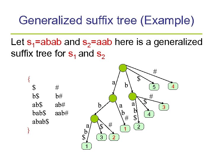
Generalized suffix tree (Example) Let s 1=abab and s 2=aab here is a generalized suffix tree for s 1 and s 2 { $ b$ ab$ bab$ abab$ } a # b# aab# b # $ 4 5 # a a $ b b 4 # $ b a b $ 1 $ # 3 1 2 2 3
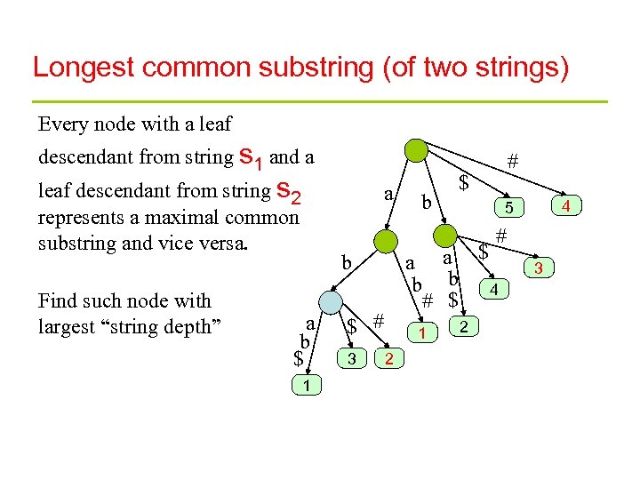
Longest common substring (of two strings) Every node with a leaf descendant from string s 1 and a leaf descendant from string s 2 represents a maximal common substring and vice versa. Find such node with largest “string depth” a b # $ 4 5 # a a $ b b 4 # $ b a b $ 1 $ # 3 1 2 2 3
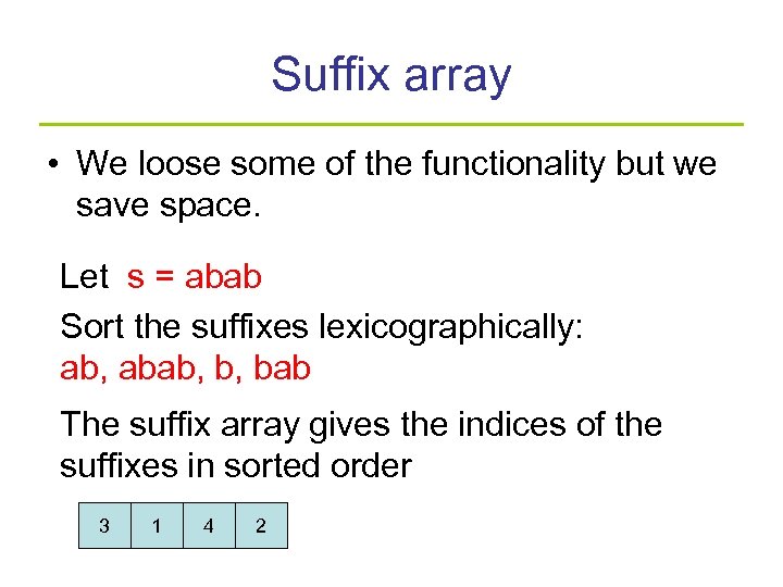
Suffix array • We loose some of the functionality but we save space. Let s = abab Sort the suffixes lexicographically: ab, abab, b, bab The suffix array gives the indices of the suffixes in sorted order 3 1 4 2
Linear time suffix array construction • Consider the popular example string S: • bananainpajamas$ 1. Construct the suffix array of S using the linear time algorithm 2. Then compute the BWT(S) 3. What’s the relationship between the suffix array and BWT ?
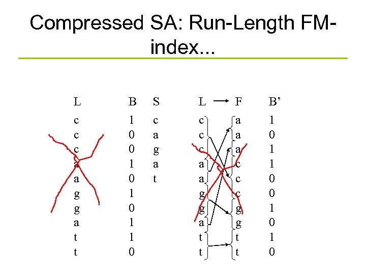
Compressed SA: Run-Length FMindex. . . L c c c a a g g a t t B 1 0 0 1 0 1 1 0 S c a g a t L c c c a a g g a t t F a a a c c c g g t t B’ 1 0 1 1 0 0 1 0
![Changes to formulas • Recall that we need to compute CT[c]+rankc(L, i) in the Changes to formulas • Recall that we need to compute CT[c]+rankc(L, i) in the](https://present5.com/presentation/73668da924f248db9b12c5d2d860aa0f/image-45.jpg)
Changes to formulas • Recall that we need to compute CT[c]+rankc(L, i) in the backward search. • Theorem: C[c]+rankc(L, i) is equivalent to select 1(B’, CS[c]+1+rankc(S, rank 1(B, i)))-1, when L[i]¹ c, and otherwise to select 1(B’, CS[c]+rankc(S, rank 1(B, i)))+ i-select 1(B, rank 1(B, i)).
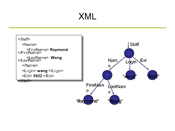
XML <Staff> <Name> <First. Name> Raymond </First. Name> <Last. Name> Wong </Last. Name> </Name> <Login> wong </Login> <Ext> 5932 </Ext> </Staff> Staff Nam e Login Ext “wong” First. Nam Last. Nam e e “Raymond” “Wong” “ 5932”
XML Parsers • There are several different ways to categorise parsers: – Validating versus non-validating parsers – Parsers that support the Document Object Model (DOM) – Parsers that support the Simple API for XML (SAX) – Parsers written in a particular language (Java, C, C++, Perl, etc. )
![XPath: More Qualifiers /bib/book[@price < “ 60”] /bib/book[author/@age < “ 25”] /bib/book[author/text()] XPath: More Qualifiers /bib/book[@price < “ 60”] /bib/book[author/@age < “ 25”] /bib/book[author/text()]](https://present5.com/presentation/73668da924f248db9b12c5d2d860aa0f/image-48.jpg)
XPath: More Qualifiers /bib/book[@price < “ 60”] /bib/book[author/@age < “ 25”] /bib/book[author/text()]
Query evaluation Top-down Bottom-up Hybrid
![XPath evaluation <a><b><c>12</c><d>7</d></b><b><c>7</c></b></a> a b b / a / b [c = “ 12”] XPath evaluation <a><b><c>12</c><d>7</d></b><b><c>7</c></b></a> a b b / a / b [c = “ 12”]](https://present5.com/presentation/73668da924f248db9b12c5d2d860aa0f/image-50.jpg)
XPath evaluation <a><b><c>12</c><d>7</d></b><b><c>7</c></b></a> a b b / a / b [c = “ 12”] c d c 12 7 7
Path indexing • Traversing graph/tree almost = query processing for semistructured / XML data • Normally, it requires to traverse the data from the root and return all nodes X reachable by a path matching the given regular path expression • Motivation: allows the system to answer regular path expressions without traversing the whole graph/tree
Two techniques • Based on the idea of languageequivalence • Data Guide
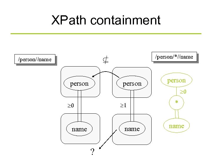
XPath containment /person//name /person/*//name person 0 1 0 name ? * name
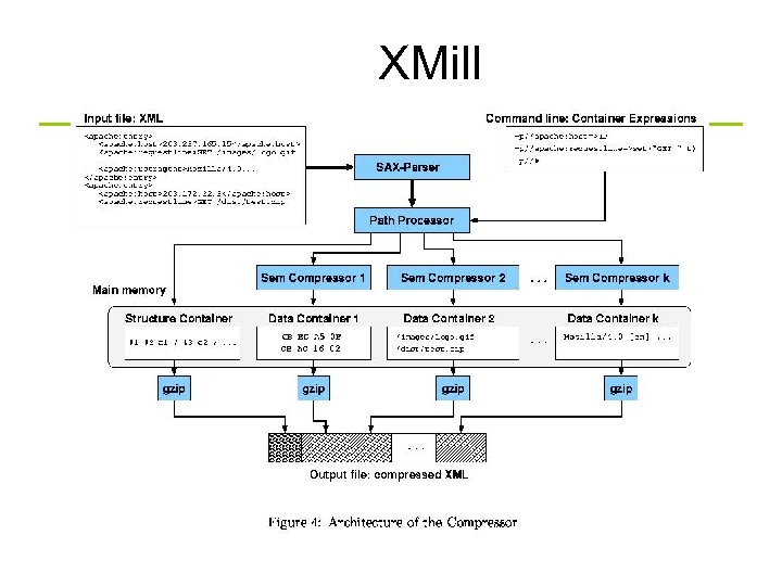
XMill
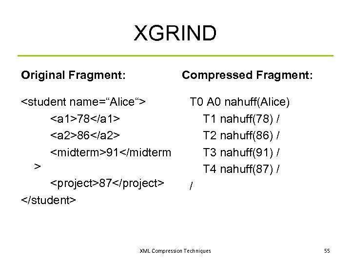
XGRIND Original Fragment: Compressed Fragment: <student name=“Alice“> <a 1>78</a 1> <a 2>86</a 2> <midterm>91</midterm > <project>87</project> </student> T 0 A 0 nahuff(Alice) T 1 nahuff(78) / T 2 nahuff(86) / T 3 nahuff(91) / T 4 nahuff(87) / / XML Compression Techniques 55
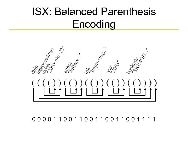
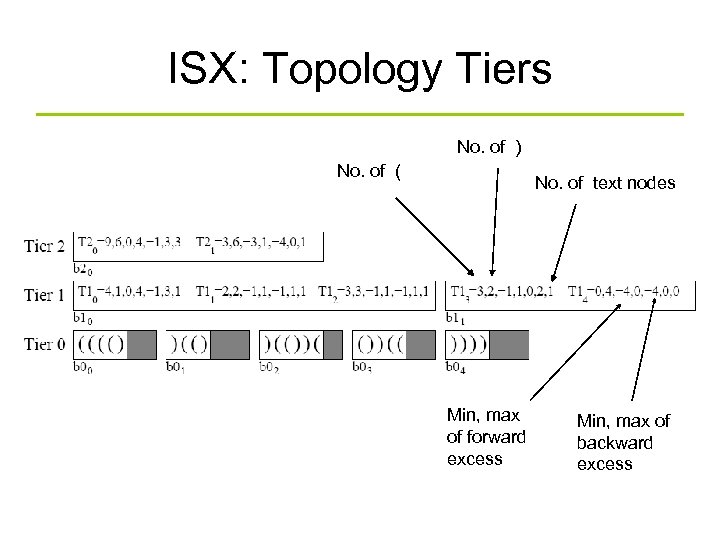
ISX: Balanced Parenthesis Encoding 0000110011001111
ISX: Topology Tiers No. of ) No. of ( No. of text nodes Min, max of forward excess Min, max of backward excess
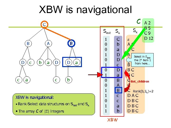
XBW is navigational C C Slast Sa B D c B A c b a a D D c a b XBW is navigational: • Rank-Select data structures on Slast and Sa • The array C of |S| integers 1 0 0 1 0 1 0 0 1 1 C b a D D c D a B A B c c a b XBW Sp A 2 B 5 C 9 D 12 e AC AC A CSelect in S last B C the 2° item 1 B C from here. . . BC BC C Get_children C C Rank(B, Sa)=2 DAC DBC DBC
![XBW is searchable (count subpaths) C C P[i+1] Slast Sa P=BD B D c XBW is searchable (count subpaths) C C P[i+1] Slast Sa P=BD B D c](https://present5.com/presentation/73668da924f248db9b12c5d2d860aa0f/image-59.jpg)
XBW is searchable (count subpaths) C C P[i+1] Slast Sa P=BD B D c A c b a a B D c D a b Inductive step: XBW the next char in Pickis searchable: P[i+1], i. e. ‘D’ • Search for data structures ‘D’ last [fr, lr] Rank-Selectthe first and last on Sin Sand Sa a • Jump to their integers Array C of |S| children fr lr 1 0 0 1 0 1 0 0 1 1 C b a D D c D a B A B c c a b A 2 B 5 C 9 D 12 Sp e AC AC AC BC BC C DA DB DB DB Rows whose Sp starts with ‘B’ Their children have upward path = ‘D B’ C C 2 occurrences of P because XBW-index of two 1 s
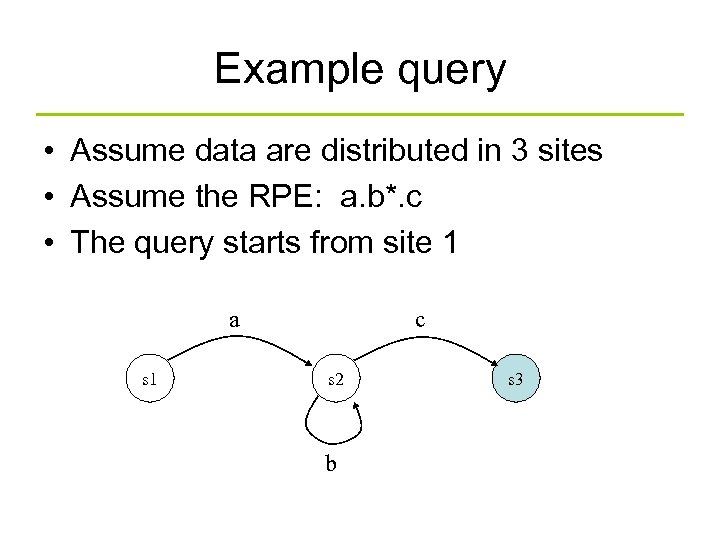
Example query • Assume data are distributed in 3 sites • Assume the RPE: a. b*. c • The query starts from site 1 a s 1 c s 2 b s 3
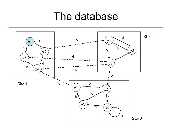
The database x 1 a y 1 b a x 2 d x 3 c b b y 3 d x 4 Site 2 d y 2 c c b Site 1 b c z 1 z 2 b b z 3 a c z 4 b Site 3
Query Processing • • Given a query, we compute its automaton Send it to each site Start an identical process at each site Compute two sets Stop(n, s) and Result(n, s) • Transmits the relations to a central location and get their union
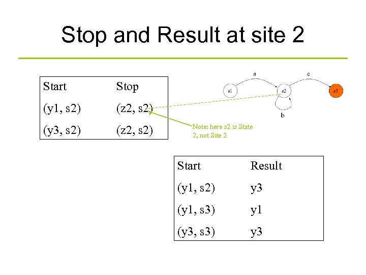
Stop and Result at site 2 Start Stop (y 1, s 2) (z 2, s 2) (y 3, s 2) (z 2, s 2) Note: here s 2 is State 2, not Site 2 Start Result (y 1, s 2) y 3 (y 1, s 3) y 1 (y 3, s 3) y 3
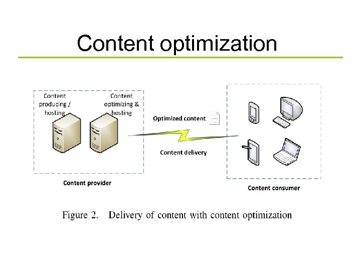
Content optimization
Web Graph Compression The compression techniques are specialized for Web Graphs. The average link size decreases with the increase of the graph. The average link access time increases with the increase of the graph. The -codes seems to have the best tradeoff between avg. bit size and access time.

Finally Course Evaluation: Much appreciated if you can provide some feedbacks to the course !!
The End kuo$cdogl
73668da924f248db9b12c5d2d860aa0f.ppt