COMP 527 Data Mining M Sulaiman Khan mskhan liv

COMP 527: Data Mining M. Sulaiman Khan (mskhan@liv. ac. uk) Dept. of Computer Science University of Liverpool 2009 ARM: Improvements March 10, 2009 Slide 1

COMP 527: Data Mining Introduction to the Course Introduction to Data Mining Introduction to Text Mining General Data Mining Issues Data Warehousing Classification: Challenges, Basics Classification: Rules Classification: Trees 2 Classification: Bayes Classification: Neural Networks Classification: SVM Classification: Evaluation 2 Regression, Prediction ARM: Improvements Input Preprocessing Attribute Selection Association Rule Mining ARM: A Priori and Data Structures ARM: Improvements ARM: Advanced Techniques Clustering: Challenges, Basics Clustering: Improvements Clustering: Advanced Algorithms Hybrid Approaches Graph Mining, Web Mining Text Mining: Challenges, Basics Text Mining: Text-as-Data Text Mining: Text-as-Language Revision for Exam March 10, 2009 Slide 2

COMP 527: Data Mining Today's Topics Sampling Negative Border Max. Miner Partitioning CLOSET ECLAT ARM: Improvements March 10, 2009 Slide 3

COMP 527: Data Mining Naïve Sampling If you could find a representative sample of the database, you could generate rules from that alone by using a reduced minimum support. Eg if you have 1 M instances, but 1000 are a true representation of those million, you could ignore the other 999, 000 and use minimum support /1000. Brilliant! Of course, it is unlikely that you'll find a representative sample, so we need some way to overcome this. Let's look at how this can be done. ARM: Improvements March 10, 2009 Slide 4

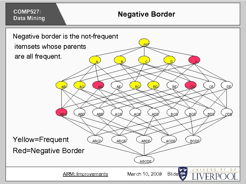COMP 527: Data Mining Negative Border Negative border is the not-frequent itemsets whose parents are all frequent. A null B C D E AB AC AD AE BC BD BE CD CE DE ABC ABD ABE ACD ACE ADE BCD BCE BDE CDE Yellow=Frequent Red=Negative Border ABCD ABCE ABDE ACDE ABCDE ARM: Improvements March 10, 2009 Slide 5 BCDE

COMP 527: Data Mining Negative Border eg: ABC is not frequent but its parents are. ABC is in the negative border. Anything below negative border must be infrequent due to downward closure. We can combine this idea with that of Sampling. . . ARM: Improvements March 10, 2009 Slide 6

COMP 527: Data Mining Sampling Instead of working with the entire database, we could use a sample of it. Then the frequent itemsets that it finds (using the reduced support threshold proportional to the sample size) are potentially frequent in the entire database. Using the negative border, we can add itemsets to these potential candidates. Suppose that {A, C, D, CD} are frequent in a sample. The border is {B, AC, AD}. The potential candidates are: {A, B, C, AD, CD} (All subsets of B are in the sample. . . eg the empty set) ARM: Improvements March 10, 2009 Slide 7

COMP 527: Data Mining Sampling Then we count against the full database. If none of the negative border itemsets are frequent, we know that none of the supersets are either. If we find that while ABC was not frequent in the sample, it was frequent in the full database, we expand the border around ABC and check again in a second pass. This makes it very likely to find all of the frequent itemsets without having to do A Priori on the entire database. But: 1. It increases the number of candidates to count in the scan through the database. 2. It's not certain of finding all frequent itemsets. ARM: Improvements March 10, 2009 Slide 8

COMP 527: Data Mining Max. Miner Similar to sampling, the Max. Miner algorithm uses the negative border. Find all frequent 1 -itemsets in a scan. eg: A, B, C, D, E Find support for patterns breadth-first (to facilitate very large databases), and prune subsets of the max pattern from future searches. Eg instead of finding AB, AC. . . AE, BC, . . . DE, if you find that BCDE is frequent pattern, then you only need to check itemsets that include 'A'. It does this by generating a set enumeration tree. . . ARM: Improvements March 10, 2009 Slide 9

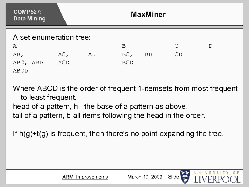COMP 527: Data Mining Max. Miner A set enumeration tree: A AB, ABC, ABD ABCD AC, ACD AD B BC, BCD BD C CD D Where ABCD is the order of frequent 1 -itemsets from most frequent to least frequent. head of a pattern, h: the base of a pattern as above. tail of a pattern, t: all items following the head in the order. If h(g)+t(g) is frequent, then there's no point expanding the tree. ARM: Improvements March 10, 2009 Slide 10

COMP 527: Data Mining Max. Miner Scan 1: Find frequent items Scan 2: Find support for potential max patterns Eg, transactions: ABCDE, ACDF Minimum Support: 2 Frequent single itemsets: ABCDE (not F) ABCDE is not frequent, but BCDE is. No need to check for CDE or CD in transaction 3 as we've already determined that BCDE is frequent. ARM: Improvements March 10, 2009 Slide 11

COMP 527: Data Mining Frequent Closed Patterns A frequent closed pattern is a frequent itemset X where no item y can be added to it, such that every transaction including X also contains y. Another way to think about it: An itemset is closed if none of its immediate supersets has the same support as the itemset. Then instead of mining everything, we only need to mine the closed patterns. All max patterns are also closed patterns, but there are closed patterns that are not max patterns. ARM: Improvements March 10, 2009 Slide 12

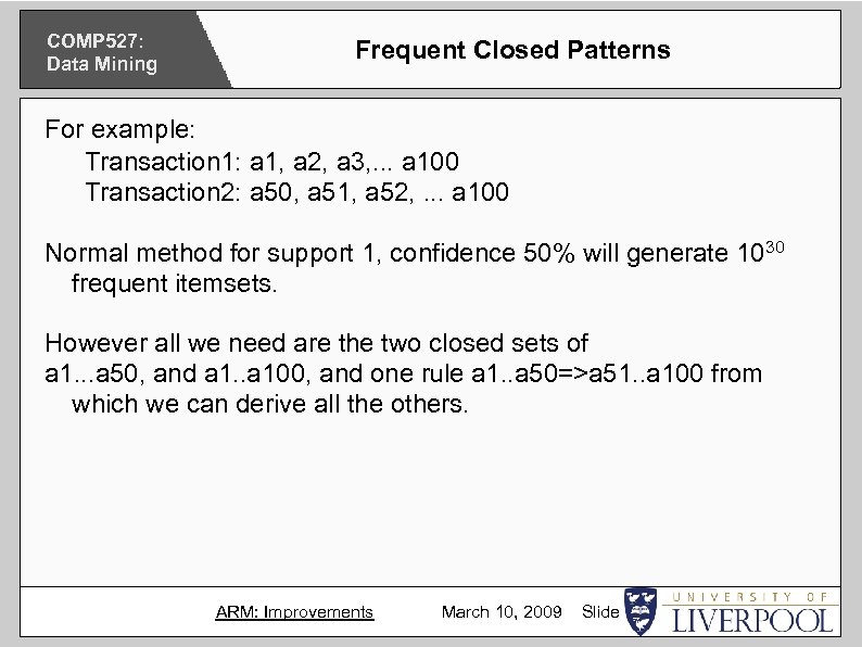COMP 527: Data Mining Frequent Closed Patterns For example: Transaction 1: a 1, a 2, a 3, . . . a 100 Transaction 2: a 50, a 51, a 52, . . . a 100 Normal method for support 1, confidence 50% will generate 1030 frequent itemsets. However all we need are the two closed sets of a 1. . . a 50, and a 1. . a 100, and one rule a 1. . a 50=>a 51. . a 100 from which we can derive all the others. ARM: Improvements March 10, 2009 Slide 13

COMP 527: Data Mining Partitioning Instead of sampling a hopefully representative portion, we could instead cut up the database into partitions such that it can be held in memory. Then we apply A Priori to each partition (without needing to go back to the disk as it's in memory) Then we have all of the itemsets that are frequent in each partition and need to merge them to generate all the frequent itemsets. All itemsets frequent (using the full minimum support) in one partition must be frequent in the entire database. All itemsets frequent (using the proportional support) in one partition may be frequent in the entire database. Itemsets not frequent in any partition must be not frequent in the database. ARM: Improvements March 10, 2009 Slide 14

COMP 527: Data Mining Partitioning So we find all check in a complete database pass all locally frequent itemsets that are not by themselves globally frequent. In this way there are only two database passes -- one to generate the partitions and one to check if locally frequent itemsets are globally frequent. And, like sampling, that is the problem with partitioning. It is likely that there will be many locally frequent itemsets that are not globally frequent, and very few locally frequent itemsets that are by themselves globally frequent. ARM: Improvements March 10, 2009 Slide 15

COMP 527: Data Mining Projected Databases Assuming that we have a fast database engine storing our transactions, at some point it may be much more efficient to step through sets of instances based on their contents, rather than all instances. find frequent 2 -itemsets. for each itemset xy, Create sub-db containing only records with that itemset Find frequent patterns in this projection and recurse if ab is frequent in the xy projection, then xyab is frequent. Better, if you know that z is not frequent, you can work with xy-z projection. Depends on the speed of your db engine. ARM: Improvements March 10, 2009 Slide 16

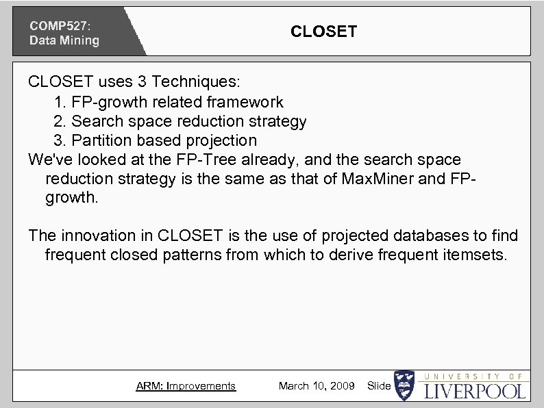COMP 527: Data Mining CLOSET uses 3 Techniques: 1. FP-growth related framework 2. Search space reduction strategy 3. Partition based projection We've looked at the FP-Tree already, and the search space reduction strategy is the same as that of Max. Miner and FPgrowth. The innovation in CLOSET is the use of projected databases to find frequent closed patterns from which to derive frequent itemsets. ARM: Improvements March 10, 2009 Slide 17

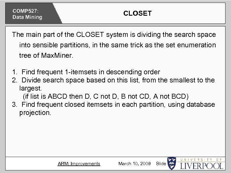COMP 527: Data Mining CLOSET The main part of the CLOSET system is dividing the search space into sensible partitions, in the same trick as the set enumeration tree of Max. Miner. 1. Find frequent 1 -itemsets in descending order 2. Divide search space based on this list, from the smallest to the largest. (if list is ABCD then D, C not D, B not CD, A not BCD) 3. Find frequent closed itemsets in each partition, using database projection. ARM: Improvements March 10, 2009 Slide 18

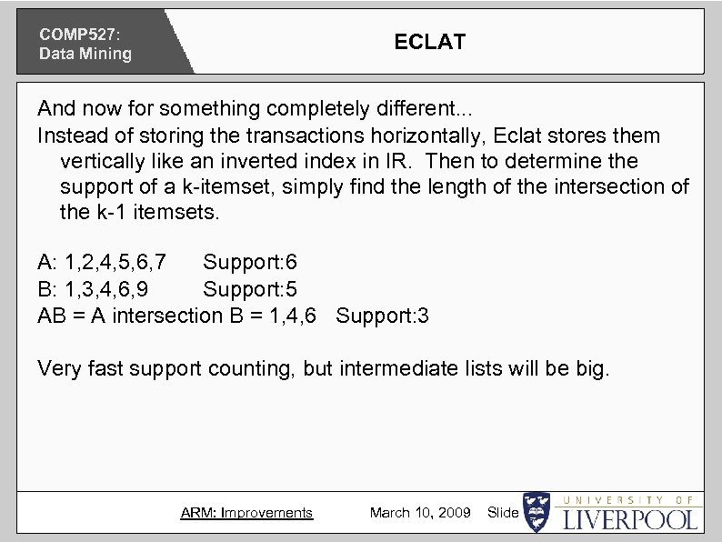COMP 527: Data Mining ECLAT And now for something completely different. . . Instead of storing the transactions horizontally, Eclat stores them vertically like an inverted index in IR. Then to determine the support of a k-itemset, simply find the length of the intersection of the k-1 itemsets. A: 1, 2, 4, 5, 6, 7 Support: 6 B: 1, 3, 4, 6, 9 Support: 5 AB = A intersection B = 1, 4, 6 Support: 3 Very fast support counting, but intermediate lists will be big. ARM: Improvements March 10, 2009 Slide 19

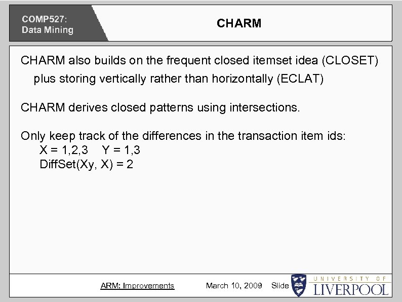COMP 527: Data Mining CHARM also builds on the frequent closed itemset idea (CLOSET) plus storing vertically rather than horizontally (ECLAT) CHARM derives closed patterns using intersections. Only keep track of the differences in the transaction item ids: X = 1, 2, 3 Y = 1, 3 Diff. Set(Xy, X) = 2 ARM: Improvements March 10, 2009 Slide 20

COMP 527: Data Mining Further Reading Dunham 6. 4 Han 5. 2 ARM: Improvements March 10, 2009 Slide 21