Combinatorial Optimization and Computer Vision Philip Torr

Story • How an attempt to solve one problem lead into many different areas of computer vision and some interesting results.

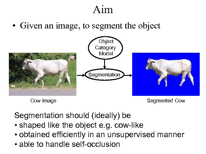
Aim • Given an image, to segment the object Object Category Model Segmentation Cow Image Segmented Cow Segmentation should (ideally) be • shaped like the object e. g. cow-like • obtained efficiently in an unsupervised manner • able to handle self-occlusion

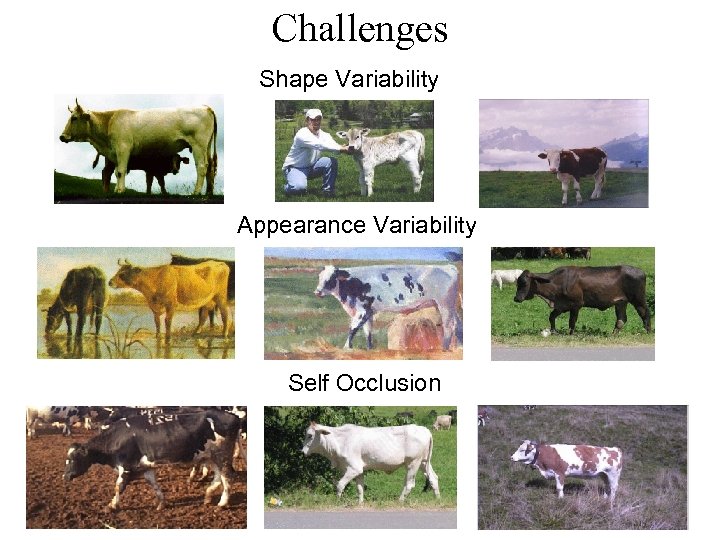
Challenges Shape Variability Appearance Variability Self Occlusion

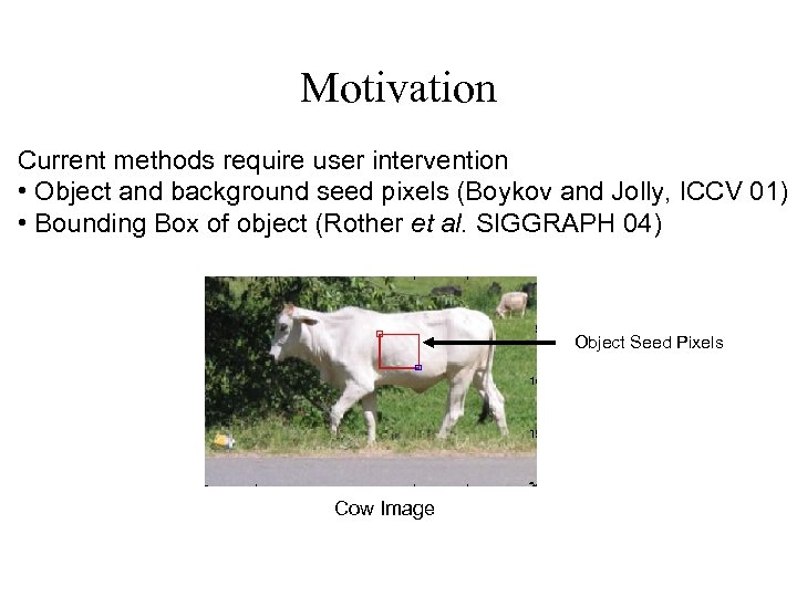
Motivation Current methods require user intervention • Object and background seed pixels (Boykov and Jolly, ICCV 01) • Bounding Box of object (Rother et al. SIGGRAPH 04) Object Seed Pixels Cow Image

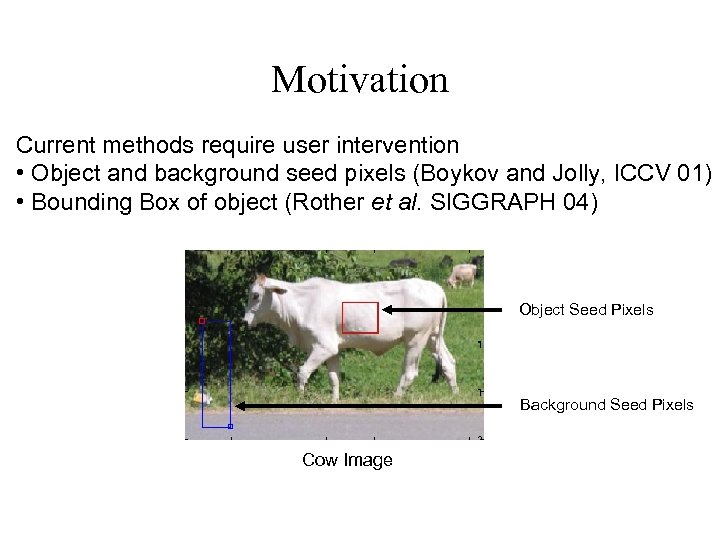
Motivation Current methods require user intervention • Object and background seed pixels (Boykov and Jolly, ICCV 01) • Bounding Box of object (Rother et al. SIGGRAPH 04) Object Seed Pixels Background Seed Pixels Cow Image

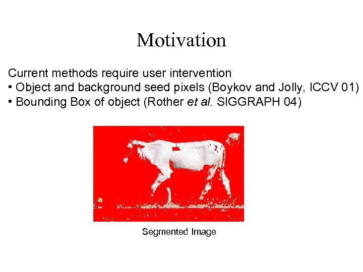
Motivation Current methods require user intervention • Object and background seed pixels (Boykov and Jolly, ICCV 01) • Bounding Box of object (Rother et al. SIGGRAPH 04) Segmented Image

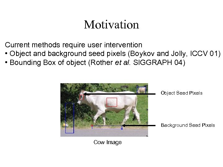
Motivation Current methods require user intervention • Object and background seed pixels (Boykov and Jolly, ICCV 01) • Bounding Box of object (Rother et al. SIGGRAPH 04) Object Seed Pixels Background Seed Pixels Cow Image

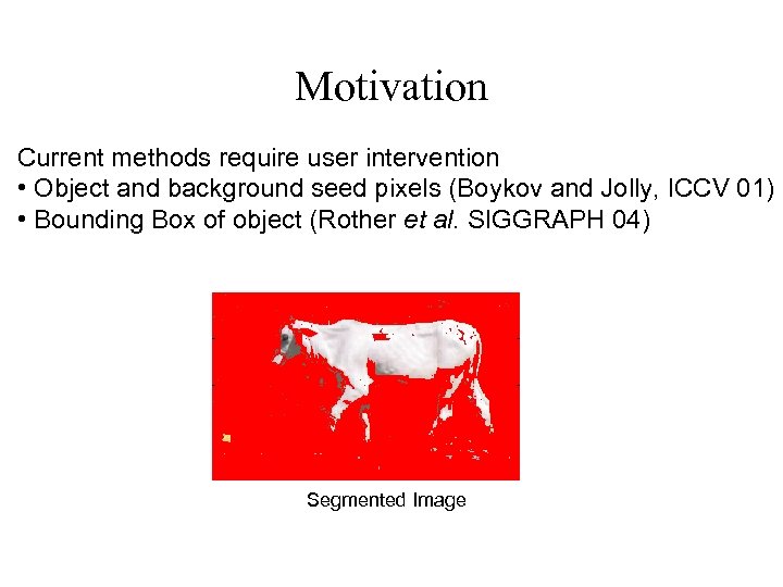
Motivation Current methods require user intervention • Object and background seed pixels (Boykov and Jolly, ICCV 01) • Bounding Box of object (Rother et al. SIGGRAPH 04) Segmented Image

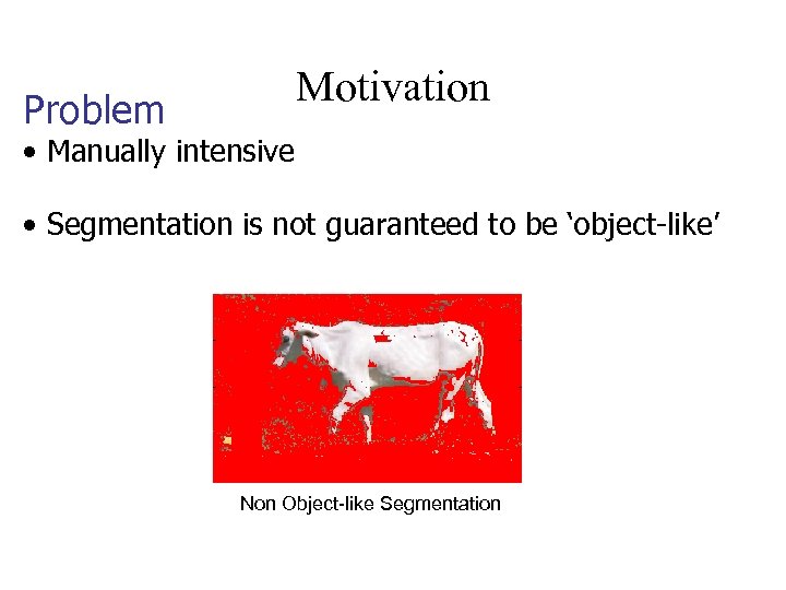
Problem Motivation • Manually intensive • Segmentation is not guaranteed to be ‘object-like’ Non Object-like Segmentation

MRF for Image Segmentation Boykov and Jolly [ICCV 2001] Energy. MRF = Unary likelihood Contrast Term Pair-wise terms (Potts Model) Maximum-a-posteriori (MAP) solution x* = arg min E(x) x Data (D) Unary likelihood Pair-wise Terms MAP Solution

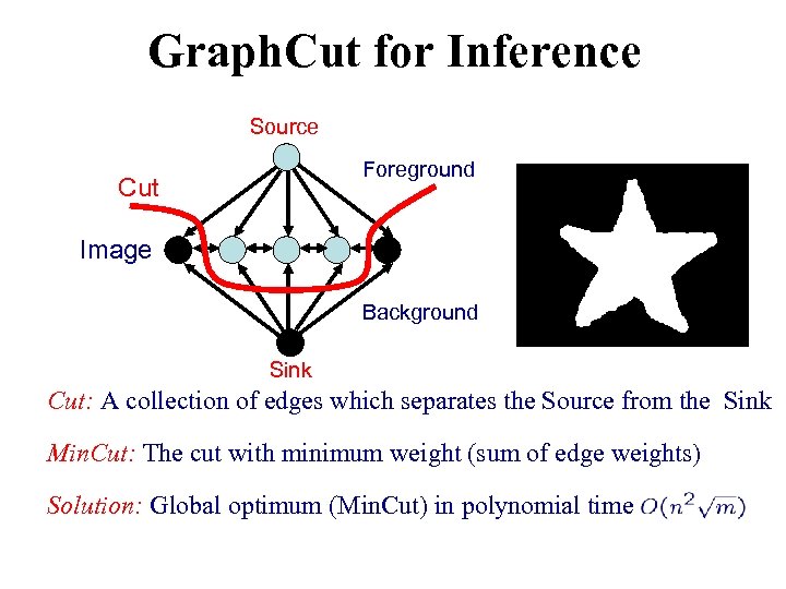
Graph. Cut for Inference Source Foreground Cut Image Background Sink Cut: A collection of edges which separates the Source from the Sink Min. Cut: The cut with minimum weight (sum of edge weights) Solution: Global optimum (Min. Cut) in polynomial time

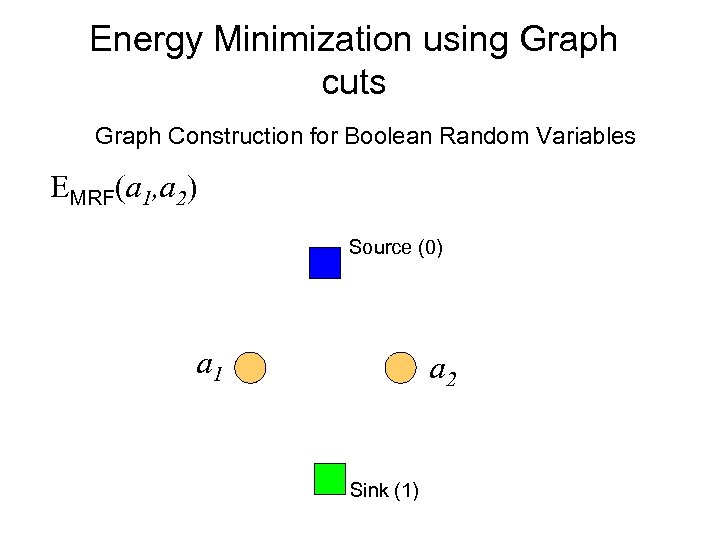
Energy Minimization using Graph cuts Graph Construction for Boolean Random Variables EMRF(a 1, a 2) Source (0) a 1 a 2 Sink (1)

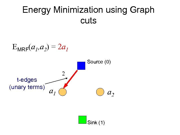
Energy Minimization using Graph cuts EMRF(a 1, a 2) = 2 a 1 Source (0) t-edges (unary terms) 2 a 1 a 2 Sink (1)

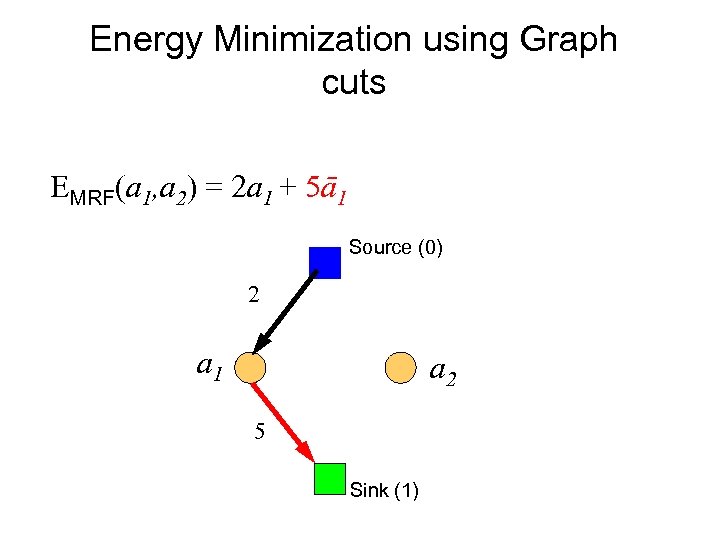
Energy Minimization using Graph cuts EMRF(a 1, a 2) = 2 a 1 + 5ā1 Source (0) 2 a 1 a 2 5 Sink (1)

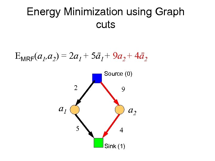
Energy Minimization using Graph cuts EMRF(a 1, a 2) = 2 a 1 + 5ā1+ 9 a 2 + 4ā2 Source (0) 2 9 a 1 a 2 5 4 Sink (1)

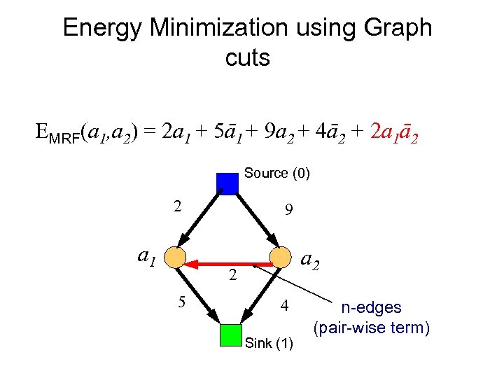
Energy Minimization using Graph cuts EMRF(a 1, a 2) = 2 a 1 + 5ā1+ 9 a 2 + 4ā2 + 2 a 1ā2 Source (0) 2 a 1 9 a 2 2 5 4 Sink (1) n-edges (pair-wise term)

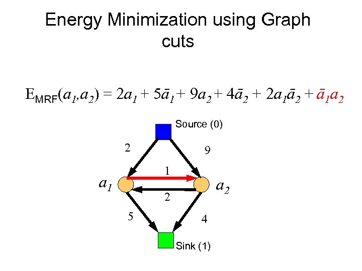
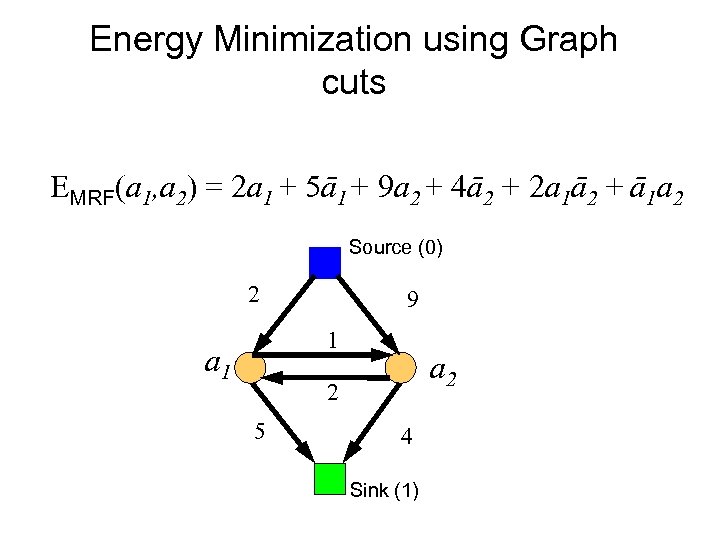
Energy Minimization using Graph cuts EMRF(a 1, a 2) = 2 a 1 + 5ā1+ 9 a 2 + 4ā2 + 2 a 1ā2 + ā1 a 2 Source (0) 2 9 1 a 2 2 5 4 Sink (1)

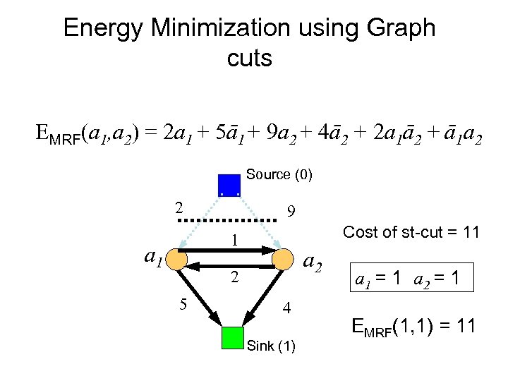
Energy Minimization using Graph cuts EMRF(a 1, a 2) = 2 a 1 + 5ā1+ 9 a 2 + 4ā2 + 2 a 1ā2 + ā1 a 2 Source (0) 2 9 Cost of st-cut = 11 1 a 2 2 5 4 Sink (1) a 1 = 1 a 2 = 1 EMRF(1, 1) = 11

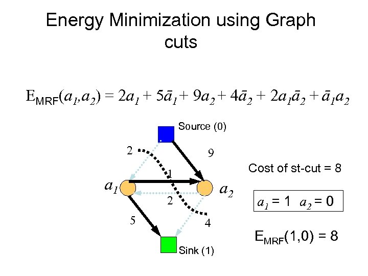
Energy Minimization using Graph cuts EMRF(a 1, a 2) = 2 a 1 + 5ā1+ 9 a 2 + 4ā2 + 2 a 1ā2 + ā1 a 2 Source (0) 2 9 Cost of st-cut = 8 1 a 2 2 5 4 Sink (1) a 1 = 1 a 2 = 0 EMRF(1, 0) = 8

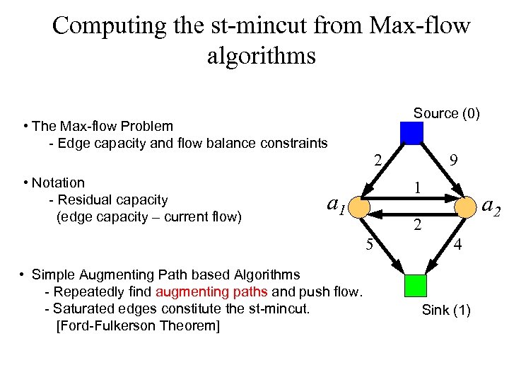
Computing the st-mincut from Max-flow algorithms • The Max-flow Problem - Edge capacity and flow balance constraints • Notation - Residual capacity (edge capacity – current flow) Source (0) 2 1 a 2 2 5 • Simple Augmenting Path based Algorithms - Repeatedly find augmenting paths and push flow. - Saturated edges constitute the st-mincut. [Ford-Fulkerson Theorem] 9 4 Sink (1)

Minimum s-t cuts algorithms n Augmenting paths [Ford & Fulkerson, 1962] n Push-relabel [Goldberg-Tarjan, 1986]

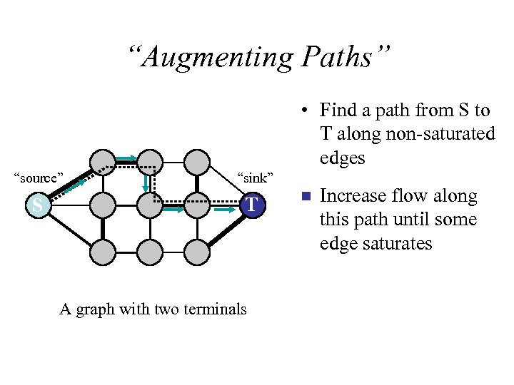
“Augmenting Paths” • Find a path from S to T along non-saturated edges “source” “sink” S T A graph with two terminals n Increase flow along this path until some edge saturates

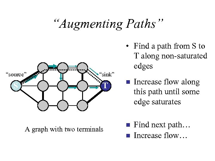
“Augmenting Paths” • Find a path from S to T along non-saturated edges “source” “sink” S T A graph with two terminals n Increase flow along this path until some edge saturates n Find next path… Increase flow… n

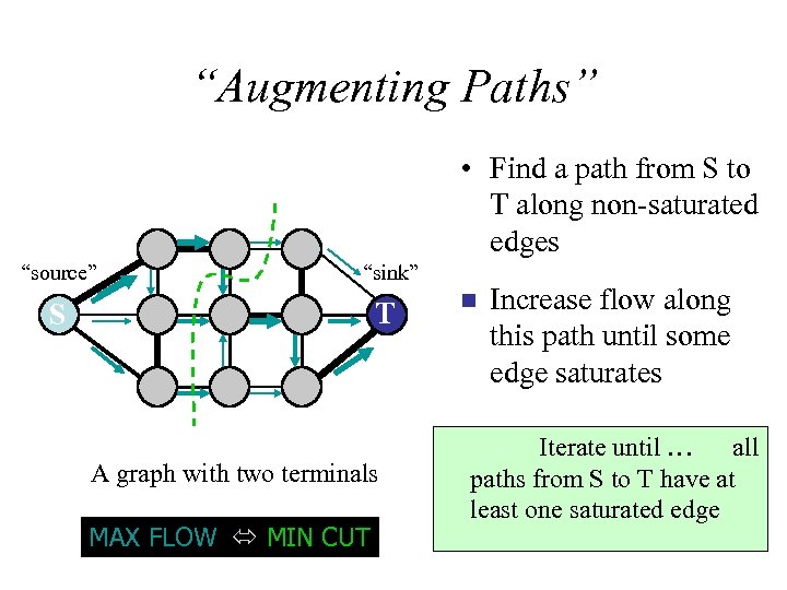
“Augmenting Paths” • Find a path from S to T along non-saturated edges “source” “sink” S T A graph with two terminals MAX FLOW MIN CUT n Increase flow along this path until some edge saturates Iterate until … all paths from S to T have at least one saturated edge

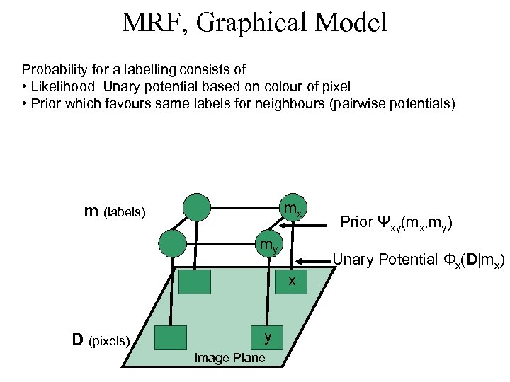
MRF, Graphical Model Probability for a labelling consists of • Likelihood Unary potential based on colour of pixel • Prior which favours same labels for neighbours (pairwise potentials) mx m (labels) my x D (pixels) y Image Plane Prior Ψxy(mx, my) Unary Potential Φx(D|mx)

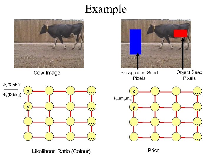
Example Cow Image Φx(D|obj) Φx(D|bkg) x Background Seed Pixels … Object Seed Pixels x … y … Ψxy(mx, my) y … … … Likelihood Ratio (Colour) Prior

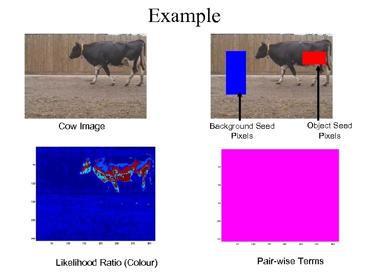
Example Cow Image Likelihood Ratio (Colour) Background Seed Pixels Object Seed Pixels Pair-wise Terms

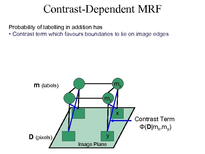
Contrast-Dependent MRF Probability of labelling in addition has • Contrast term which favours boundaries to lie on image edges mx m (labels) my x D (pixels) y Image Plane Contrast Term Φ(D|mx, my)

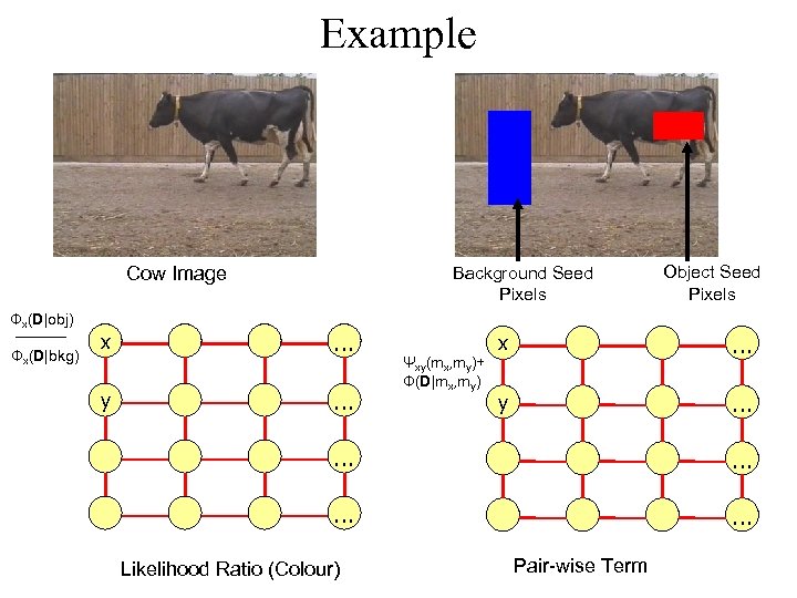
Example Cow Image Φx(D|obj) Φx(D|bkg) x y Background Seed Pixels … … Ψxy(mx, my)+ Φ(D|mx, my) Object Seed Pixels x … y … … … Likelihood Ratio (Colour) Pair-wise Term

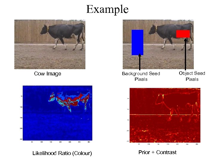
Example Cow Image Likelihood Ratio (Colour) Background Seed Pixels Prior + Contrast Object Seed Pixels

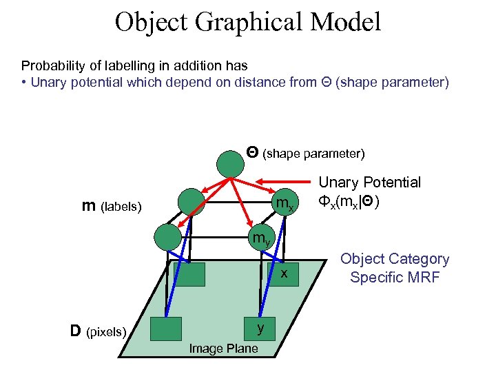
Object Graphical Model Probability of labelling in addition has • Unary potential which depend on distance from Θ (shape parameter) mx m (labels) Unary Potential Φx(mx|Θ) my x D (pixels) y Image Plane Object Category Specific MRF

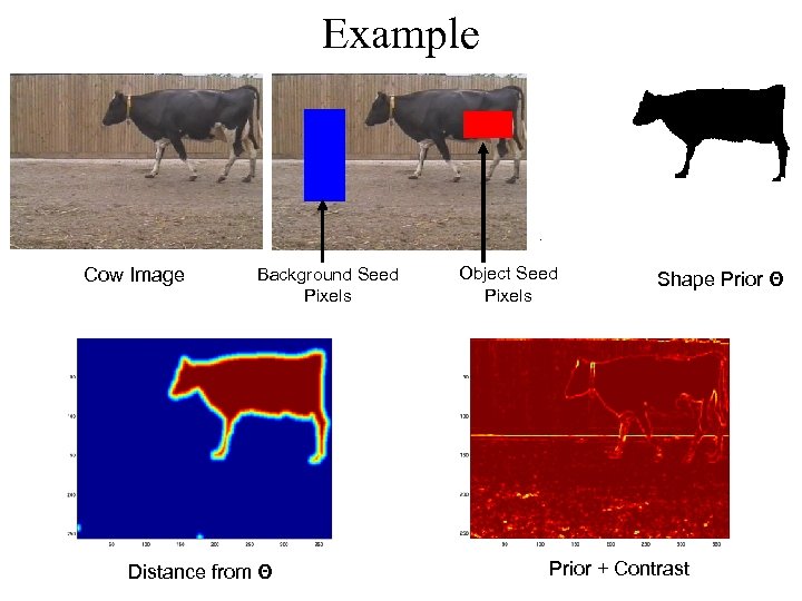
Example Cow Image Background Seed Pixels Distance from Θ Object Seed Pixels Shape Prior Θ Prior + Contrast

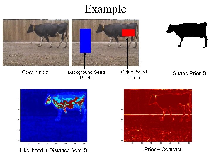
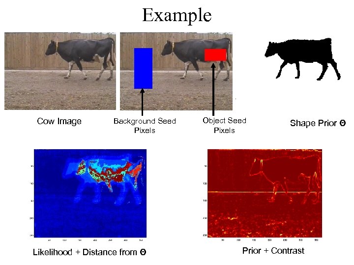
Example Cow Image Background Seed Pixels Likelihood + Distance from Θ Object Seed Pixels Shape Prior Θ Prior + Contrast

Thought • We can imagine rather than using user input to define histograms we use object detection.

Shape Model • BMVC 2004

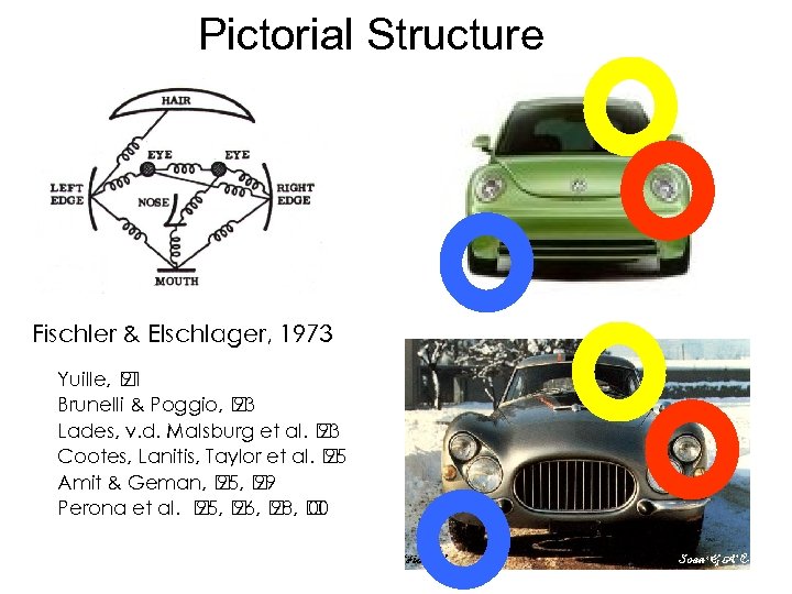
Pictorial Structure Fischler & Elschlager, 1973 f f f Yuille, 91 Brunelli & Poggio, 93 Lades, v. d. Malsburg et al. 93 Cootes, Lanitis, Taylor et al. 95 Amit & Geman, 95, 99 Perona et al. 95, 96, 98, 00

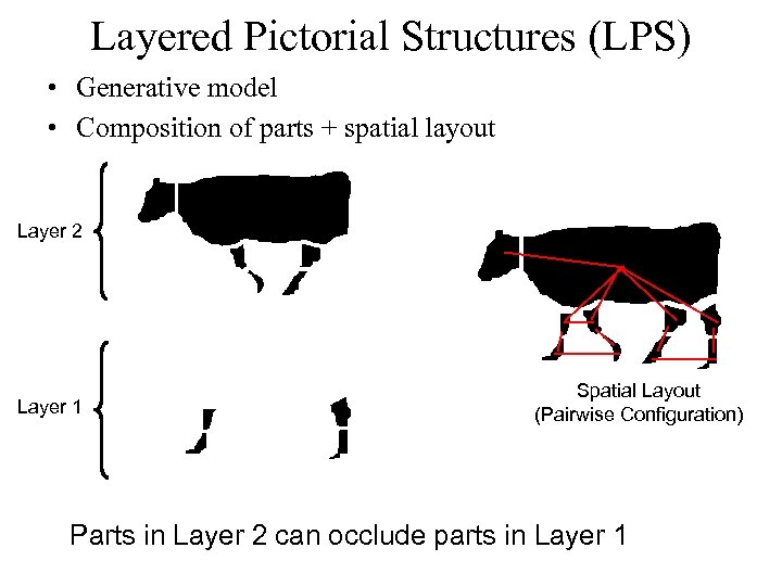
Layered Pictorial Structures (LPS) • Generative model • Composition of parts + spatial layout Layer 2 Layer 1 Spatial Layout (Pairwise Configuration) Parts in Layer 2 can occlude parts in Layer 1

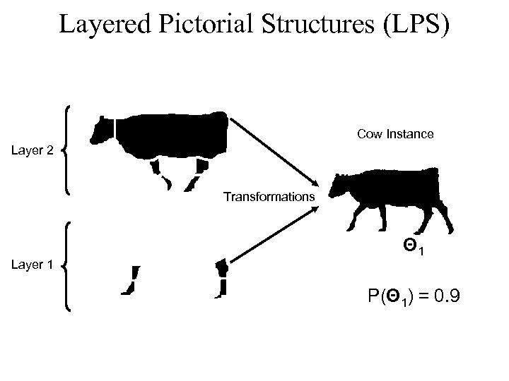
Layered Pictorial Structures (LPS) Cow Instance Layer 2 Transformations Layer 1 Θ 1 P(Θ 1) = 0. 9

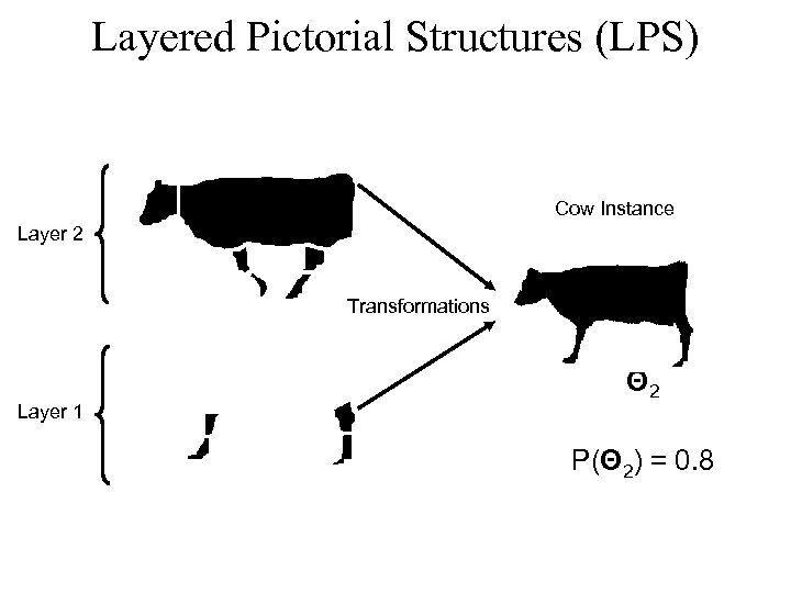
Layered Pictorial Structures (LPS) Cow Instance Layer 2 Transformations Layer 1 Θ 2 P(Θ 2) = 0. 8

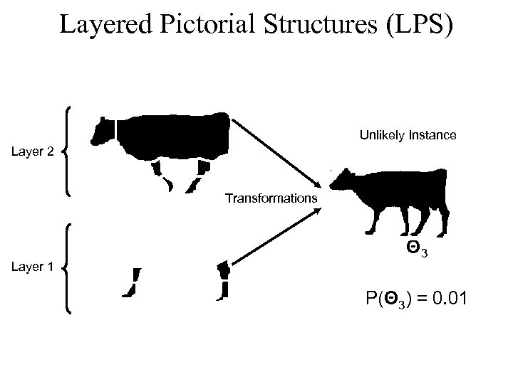
Layered Pictorial Structures (LPS) Unlikely Instance Layer 2 Transformations Layer 1 Θ 3 P(Θ 3) = 0. 01

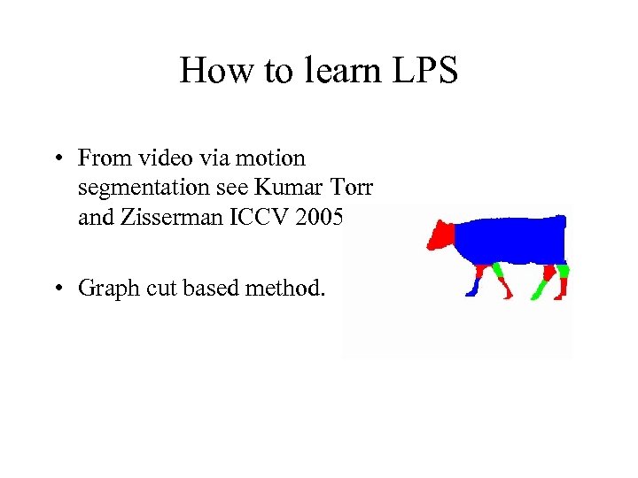
How to learn LPS • From video via motion segmentation see Kumar Torr and Zisserman ICCV 2005. • Graph cut based method.

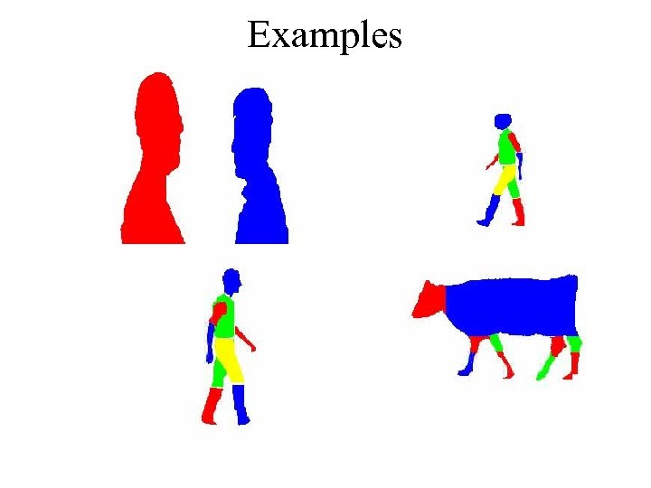
Examples

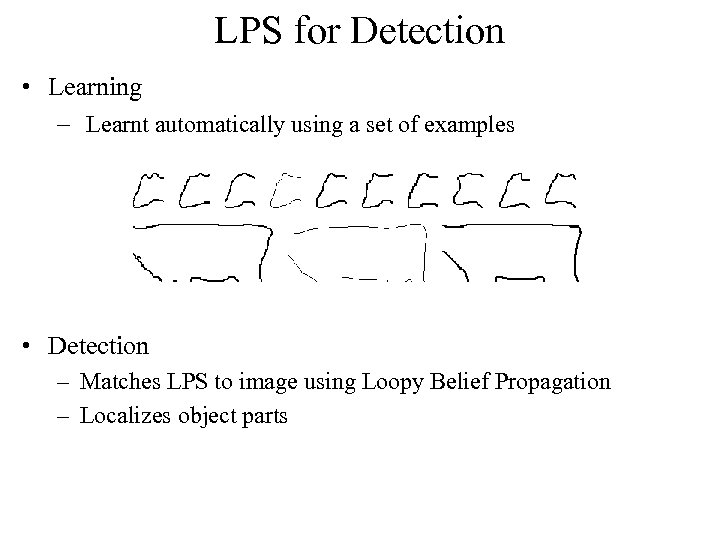
LPS for Detection • Learning – Learnt automatically using a set of examples • Detection – Matches LPS to image using Loopy Belief Propagation – Localizes object parts

Detection • Like a proposal process.

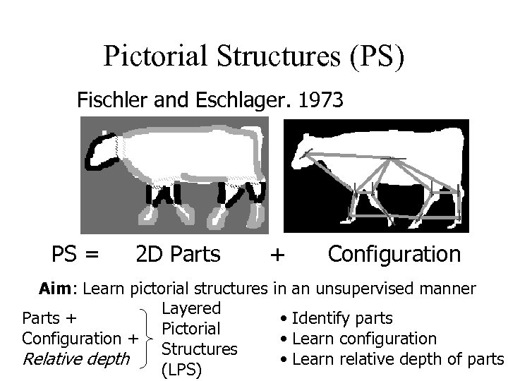
Pictorial Structures (PS) Fischler and Eschlager. 1973 PS = 2 D Parts Aim: Learn pictorial structures Layered Parts + Pictorial Configuration + Structures Relative depth (LPS) + Configuration in an unsupervised manner • Identify parts • Learn configuration • Learn relative depth of parts

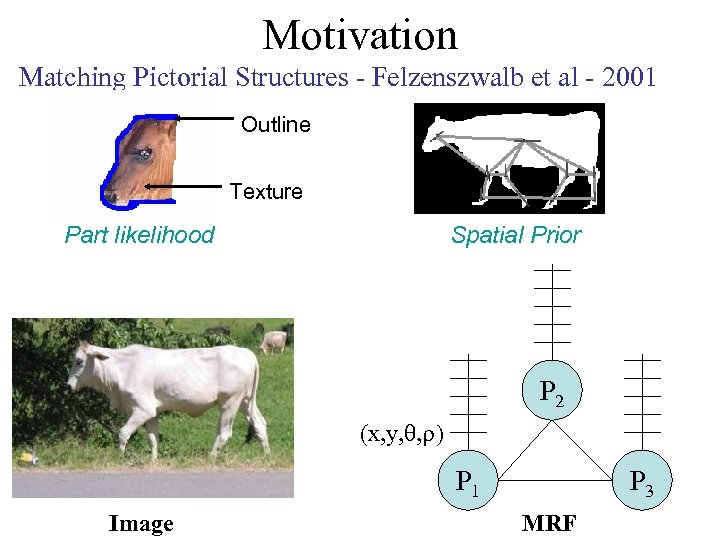
Motivation Matching Pictorial Structures - Felzenszwalb et al - 2001 Outline Texture Part likelihood Spatial Prior P 2 (x, y, , ) P 1 Image P 3 MRF

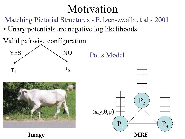
Motivation Matching Pictorial Structures - Felzenszwalb et al - 2001 • Unary potentials are negative log likelihoods Valid pairwise configuration YES NO 1 2 Potts Model P 2 (x, y, , ) P 1 Image P 3 MRF

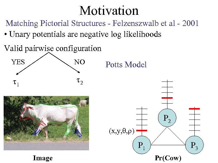
Motivation Matching Pictorial Structures - Felzenszwalb et al - 2001 • Unary potentials are negative log likelihoods Valid pairwise configuration YES NO 1 2 Potts Model P 2 (x, y, , ) P 1 Image P 3 Pr(Cow)

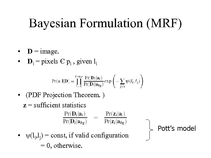
Bayesian Formulation (MRF) • D = image. • Di = pixels Є pi , given li • (PDF Projection Theorem. ) z = sufficient statistics • ψ(li, lj) = const, if valid configuration = 0, otherwise. Pott’s model

Combinatorial Optimization • SDP formulation (Torr 2001, AI stats), best bound • SOCP formulation (Kumar, Torr & Zisserman this conference), good compromise of speed and accuracy. • LBP (Huttenlocher, many), worst bound.

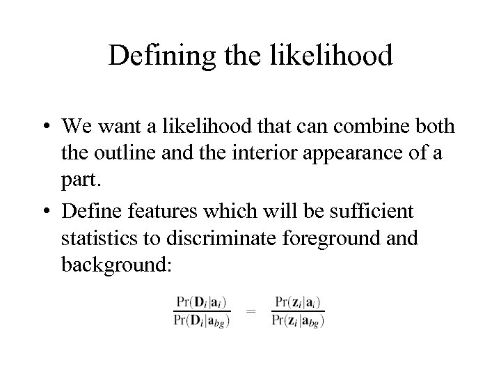
Defining the likelihood • We want a likelihood that can combine both the outline and the interior appearance of a part. • Define features which will be sufficient statistics to discriminate foreground and background:

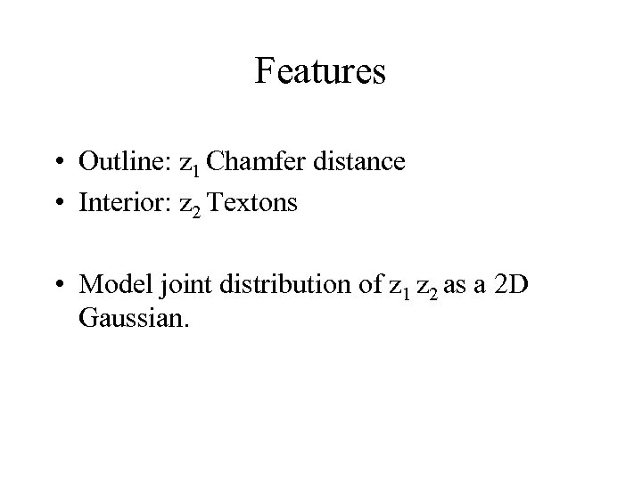
Features • Outline: z 1 Chamfer distance • Interior: z 2 Textons • Model joint distribution of z 1 z 2 as a 2 D Gaussian.

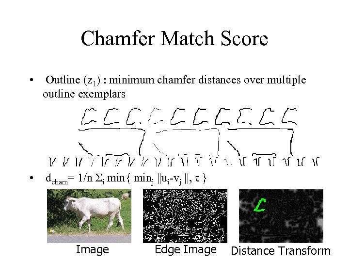
Chamfer Match Score • Outline (z 1) : minimum chamfer distances over multiple outline exemplars • dcham= 1/n Σi min{ minj ||ui-vj ||, τ } Image Edge Image Distance Transform

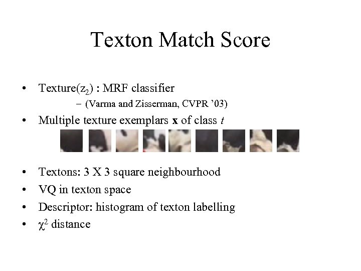
Texton Match Score • Texture(z 2) : MRF classifier – (Varma and Zisserman, CVPR ’ 03) • Multiple texture exemplars x of class t • • Textons: 3 X 3 square neighbourhood VQ in texton space Descriptor: histogram of texton labelling χ2 distance

Bag of Words/Histogram of Textons • Having slagged off Bo. W’s I reveal we used it all along, no big deal. • So this is like a spatially aware bag of words model… • Using a spatially flexible set of templates to work out our bag of words.

2. Fitting the Model • Cascades of classifiers – Efficient likelihood evaluation • Solving MRF – LBP, use fast algorithm – GBP if LBP doesn’t converge – Could use Semi Definite Programming (2003) – Recent work second order cone programming method best CVPR 2006.

Efficient Detection of parts • Cascade of classifiers • Top level use chamfer and distance transform for efficient pre filtering • At lower level use full texture model for verification, using efficient nearest neighbour speed ups.

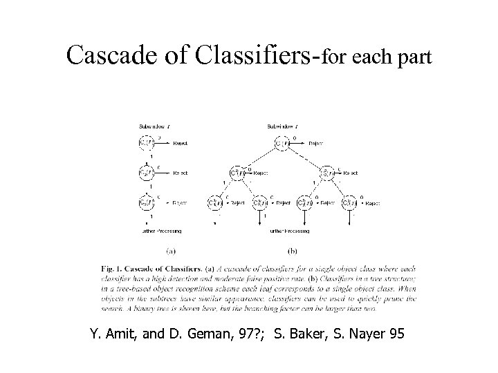
Cascade of Classifiers-for each part f. Y. Amit, and D. Geman, 97? ; S. Baker, S. Nayer 95

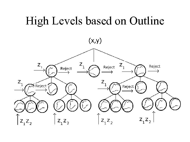
High Levels based on Outline (x, y)

Low levels on Texture • The top levels of the tree use outline to eliminate patches of the image. • Efficiency: Using chamfer distance and pre computed distance map. • Remaining candidates evaluated using full texture model.

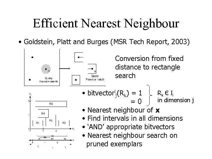
Efficient Nearest Neighbour • Goldstein, Platt and Burges (MSR Tech Report, 2003) Conversion from fixed distance to rectangle search Rk Є I i • bitvectorij(Rk) = 1 in dimension j =0 • Nearest neighbour of x • Find intervals in all dimensions • ‘AND’ appropriate bitvectors • Nearest neighbour search on pruned exemplars

Inspiration • ICCV 2003, Stenger et al. • System developed for tracking articulated objects such as hands or bodies, based on efficient detection.

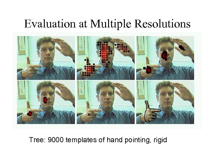
Evaluation at Multiple Resolutions Tree: 9000 templates of hand pointing, rigid

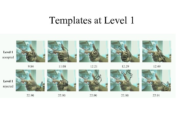
Templates at Level 1

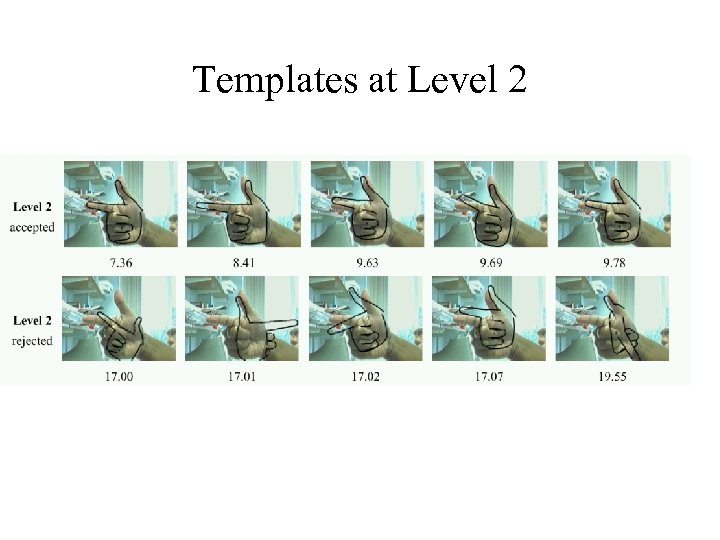
Templates at Level 2

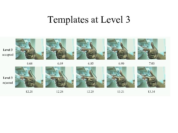
Templates at Level 3

Tracking Results

Marginalize out Pose • Get an initial estimate of pose distribution. • Use EM to marginalize out pose.

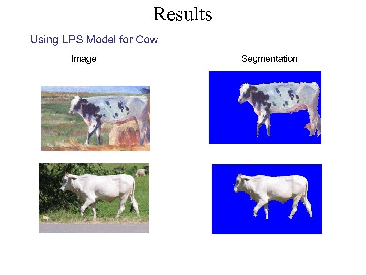
Results Using LPS Model for Cow Image Segmentation

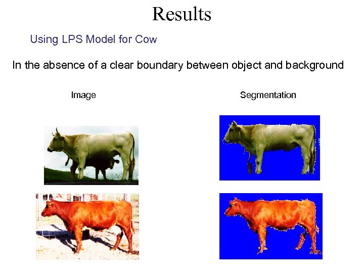
Results Using LPS Model for Cow In the absence of a clear boundary between object and background Image Segmentation

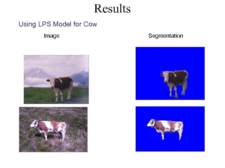
Results Using LPS Model for Cow Image Segmentation

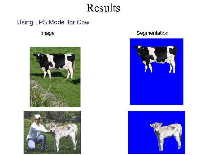
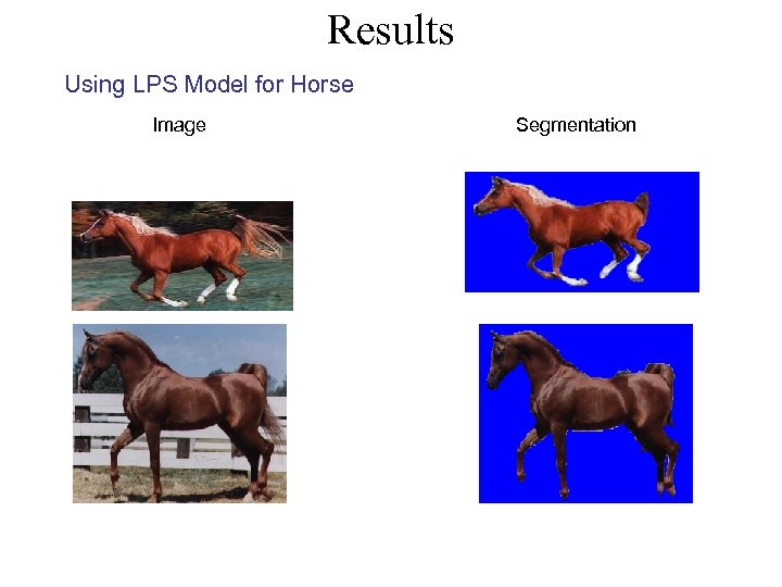
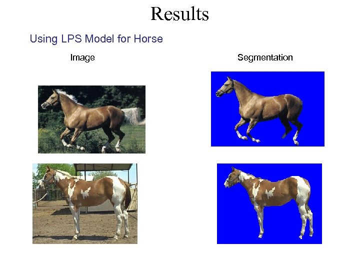
Results Using LPS Model for Horse Image Segmentation

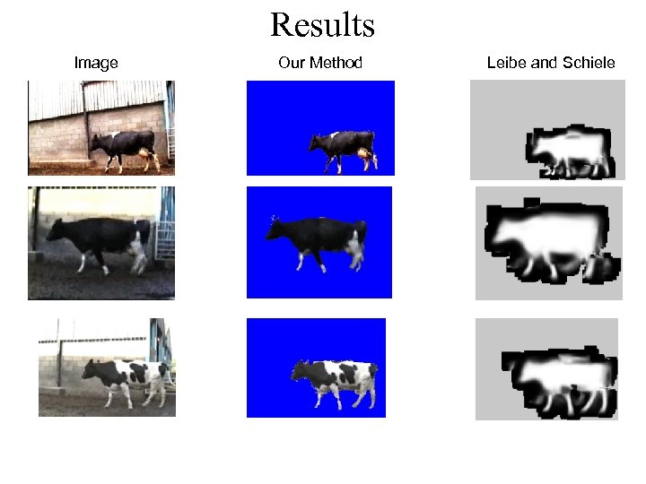
Results Image Our Method Leibe and Schiele

Thoughts Object models can help segmentation. But good models hard to obtain.

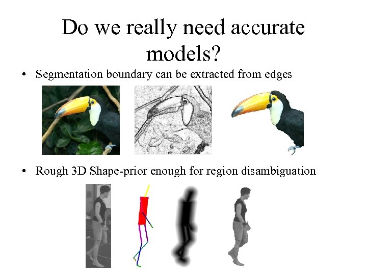
Do we really need accurate models? • Segmentation boundary can be extracted from edges • Rough 3 D Shape-prior enough for region disambiguation

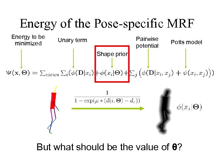
Energy of the Pose-specific MRF Energy to be minimized Pairwise potential Unary term Potts model Shape prior But what should be the value of θ?

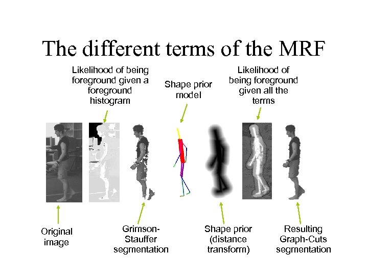
The different terms of the MRF Likelihood of being foreground given a foreground histogram Original image Shape prior model Grimson. Stauffer segmentation Likelihood of being foreground given all the terms Shape prior (distance transform) Resulting Graph-Cuts segmentation

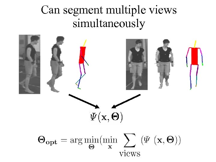
Can segment multiple views simultaneously

Solve via gradient descent • Comparable to level set methods • Could use other approaches (e. g. Objcut) • Need a graph cut per function evaluation

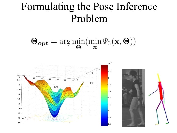
Formulating the Pose Inference Problem

But… … to compute the MAP of E(x) w. r. t the pose, it means that the unary terms will be changed at EACH iteration and the maxflow recomputed! However… n Kohli and Torr showed how dynamic graph cuts can be used to efficiently find MAP solutions for MRFs that change minimally from one time instant to the next: Dynamic Graph Cuts (ICCV 05).

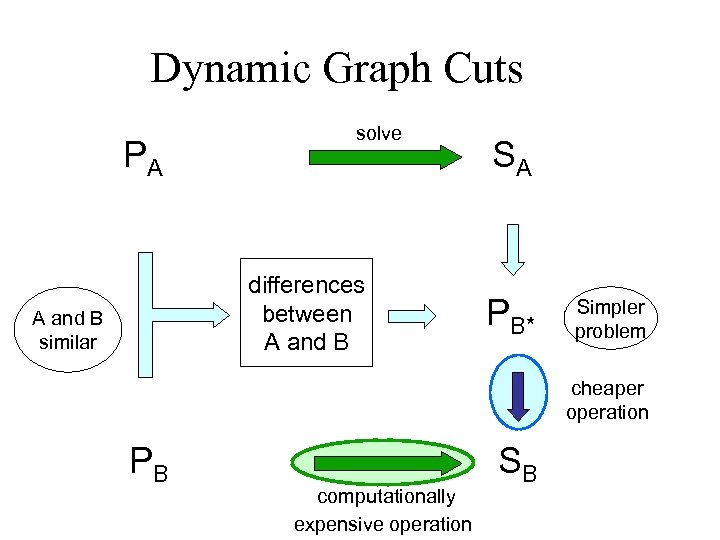
Dynamic Graph Cuts PA solve differences between A and B similar SA PB* Simpler problem cheaper operation PB computationally expensive operation SB

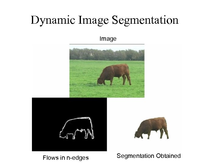
Dynamic Image Segmentation Image Flows in n-edges Segmentation Obtained

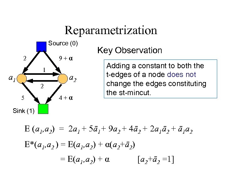
Reparametrization Source (0) 9+α 2 1 a 1 2 5 a 2 4+α Key Observation Adding a constant to both the t-edges of a node does not change the edges constituting the st-mincut. Sink (1) E (a 1, a 2) = 2 a 1 + 5ā1+ 9 a 2 + 4ā2 + 2 a 1ā2 + ā1 a 2 E*(a 1, a 2 ) = E(a 1, a 2) + α(a 2+ā2) = E(a 1, a 2) + α [a 2+ā2 =1]

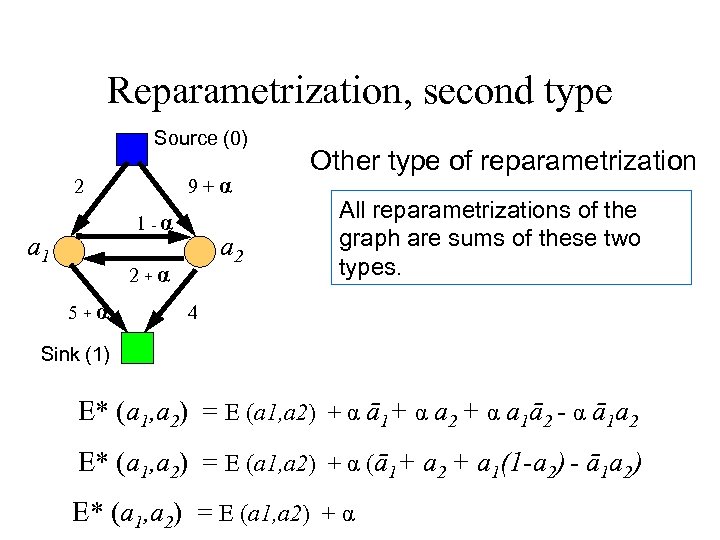
Reparametrization, second type Source (0) 9+α 2 1 -α a 1 a 2 2+α 5+α Other type of reparametrization All reparametrizations of the graph are sums of these two types. 4 Sink (1) E* (a 1, a 2) = E (a 1, a 2) + α ā1+ α a 2 + α a 1ā2 - α ā1 a 2 E* (a 1, a 2) = E (a 1, a 2) + α (ā1+ a 2 + a 1(1 -a 2) - ā1 a 2) E* (a 1, a 2) = E (a 1, a 2) + α

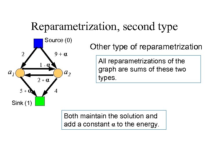
Reparametrization, second type Source (0) 9+α 2 1 -α a 1 a 2 2+α 5+α Other type of reparametrization All reparametrizations of the graph are sums of these two types. 4 Sink (1) Both maintain the solution and add a constant α to the energy.

Reparametrization • Nice result (easy to prove) • All other reparametrizations can be viewed in terms of these two basic operations. • Proof in Hammer, and also in one of Vlad’s recent papers.

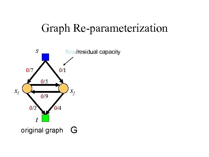
Graph Re-parameterization s flow/residual capacity 0/7 0/1 0/5 xi xj 0/9 0/2 0/4 t original graph G

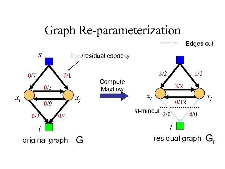
Graph Re-parameterization Edges cut s flow/residual capacity 0/7 5/2 0/1 Compute Maxflow 0/5 xi xj 0/9 0/2 xi xj 0/12 2/0 4/0 t t original graph 3/2 st-mincut 0/4 1/0 G residual graph Gr

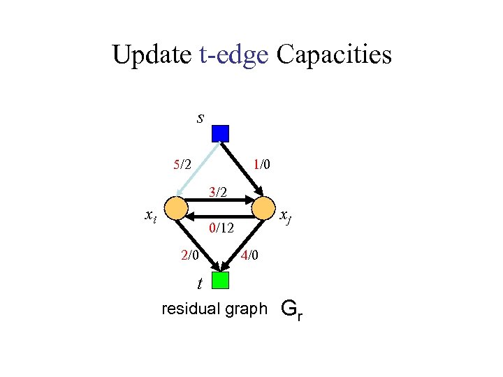
Update t-edge Capacities s 5/2 1/0 3/2 xi xj 0/12 2/0 4/0 t residual graph Gr

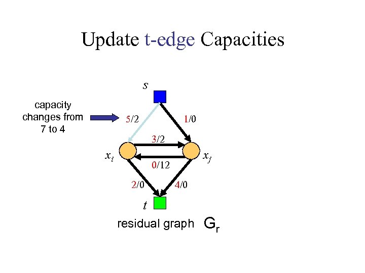
Update t-edge Capacities s capacity changes from 7 to 4 5/2 1/0 3/2 xi xj 0/12 2/0 4/0 t residual graph Gr

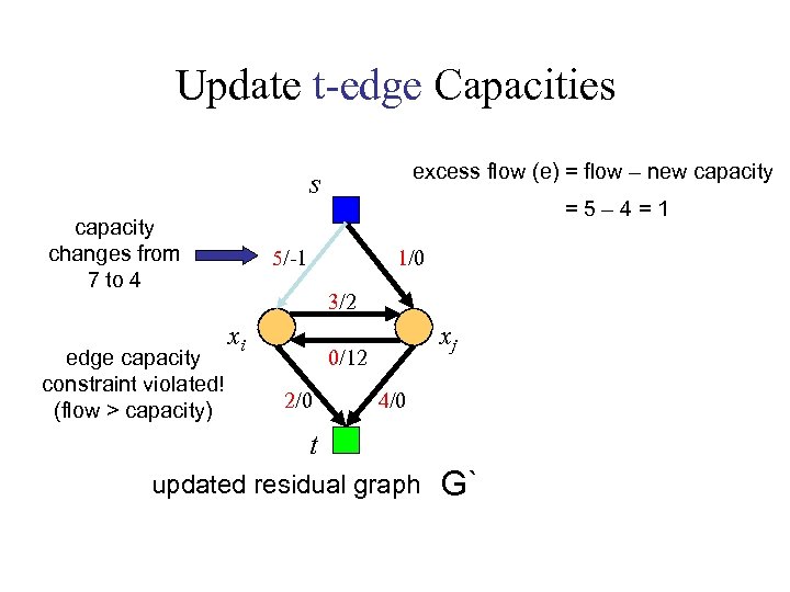
Update t-edge Capacities excess flow (e) = flow – new capacity s capacity changes from 7 to 4 edge capacity constraint violated! (flow > capacity) =5– 4=1 5/-1 1/0 3/2 xi xj 0/12 2/0 4/0 t updated residual graph G`

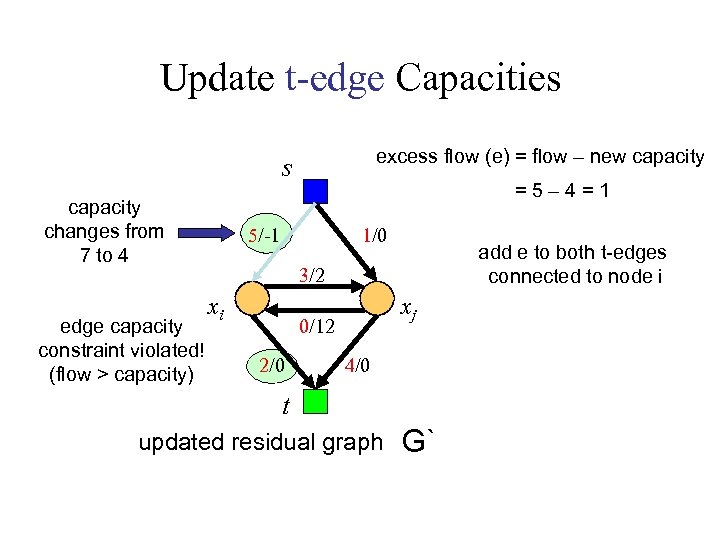
Update t-edge Capacities excess flow (e) = flow – new capacity s capacity changes from 7 to 4 edge capacity constraint violated! (flow > capacity) =5– 4=1 5/-1 1/0 add e to both t-edges connected to node i 3/2 xi xj 0/12 2/0 4/0 t updated residual graph G`

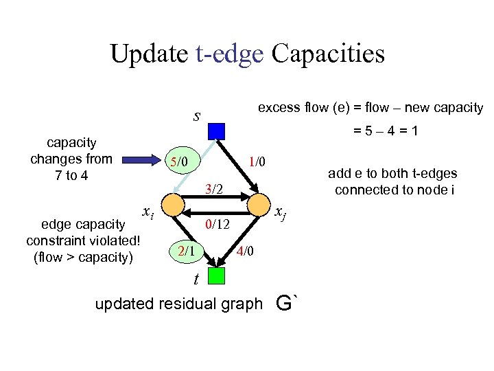
Update t-edge Capacities excess flow (e) = flow – new capacity s capacity changes from 7 to 4 edge capacity constraint violated! (flow > capacity) =5– 4=1 5/0 1/0 add e to both t-edges connected to node i 3/2 xi xj 0/12 2/1 4/0 t updated residual graph G`

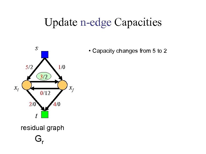
Update n-edge Capacities s • Capacity changes from 5 to 2 5/2 1/0 3/2 xi xj 0/12 2/0 4/0 t residual graph Gr

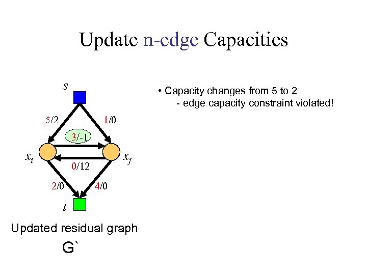
Update n-edge Capacities s • Capacity changes from 5 to 2 - edge capacity constraint violated! 5/2 1/0 3/-1 xi xj 0/12 2/0 4/0 t Updated residual graph G`

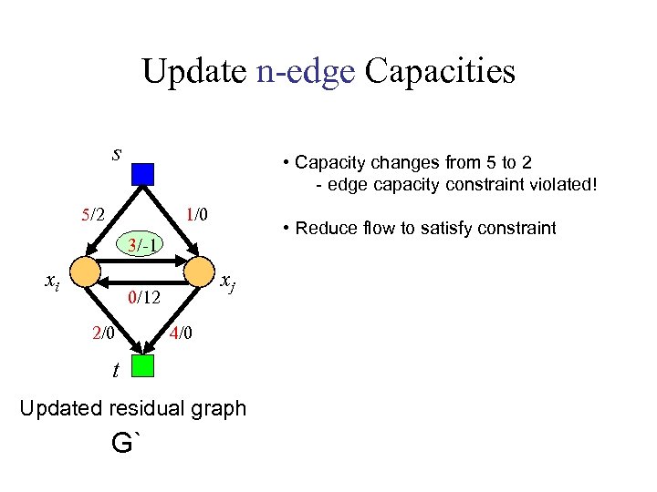
Update n-edge Capacities s • Capacity changes from 5 to 2 - edge capacity constraint violated! 5/2 1/0 • Reduce flow to satisfy constraint 3/-1 xi xj 0/12 2/0 4/0 t Updated residual graph G`

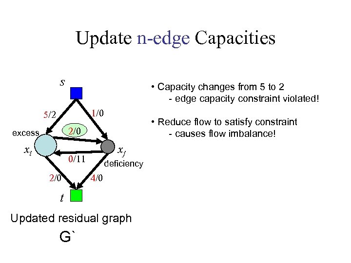
Update n-edge Capacities s • Capacity changes from 5 to 2 - edge capacity constraint violated! 1/0 5/2 • Reduce flow to satisfy constraint - causes flow imbalance! 2/0 excess xi xj 0/11 2/0 deficiency 4/0 t Updated residual graph G`

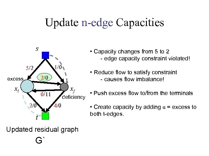
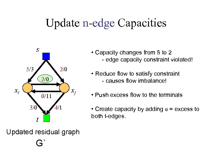
Update n-edge Capacities s • Capacity changes from 5 to 2 - edge capacity constraint violated! 1/0 5/2 • Reduce flow to satisfy constraint - causes flow imbalance! 2/0 excess xi xj 0/11 2/0 deficiency 4/0 t Updated residual graph G` • Push excess flow to/from the terminals • Create capacity by adding α = excess to both t-edges.

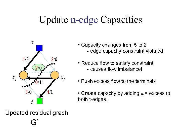
Update n-edge Capacities s • Capacity changes from 5 to 2 - edge capacity constraint violated! 5/3 2/0 • Reduce flow to satisfy constraint - causes flow imbalance! 2/0 xi xj 0/11 3/0 4/1 t Updated residual graph G` • Push excess flow to the terminals • Create capacity by adding α = excess to both t-edges.

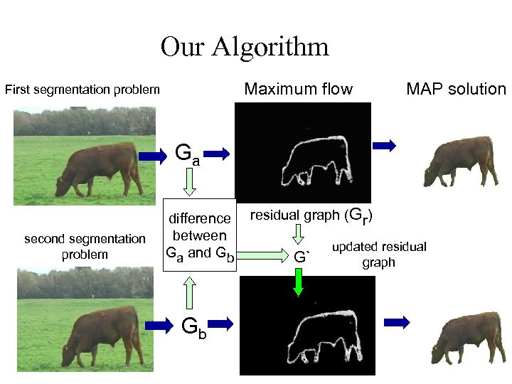
Our Algorithm Maximum flow First segmentation problem MAP solution Ga second segmentation problem difference between Ga and Gb Gb residual graph (Gr) G` updated residual graph

Dynamic Graph Cut vs Active Cuts • Our method flow recycling • AC cut recycling • Both methods: Tree recycling

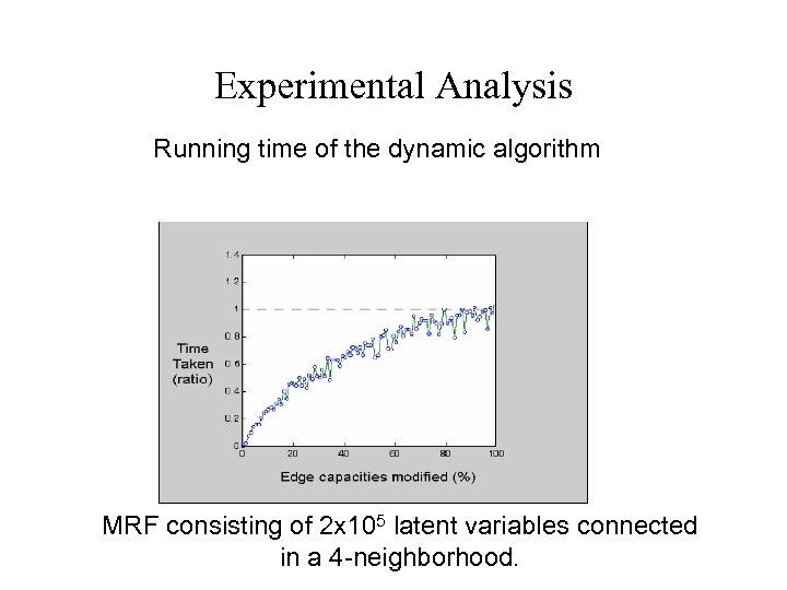
Experimental Analysis Running time of the dynamic algorithm MRF consisting of 2 x 105 latent variables connected in a 4 -neighborhood.

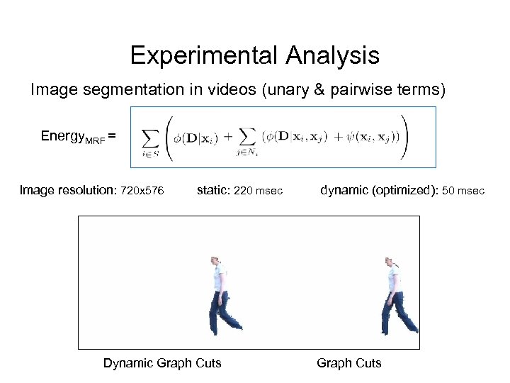
Experimental Analysis Image segmentation in videos (unary & pairwise terms) Energy. MRF = Image resolution: 720 x 576 static: 220 msec Dynamic Graph Cuts dynamic (optimized): 50 msec Graph Cuts

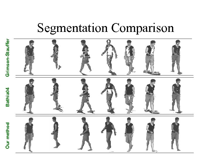
Our method Bathia 04 Grimson-Stauffer Segmentation Comparison

Segmentation + Pose inference [Images courtesy: M. Black, L. Sigal]

Segmentation + Pose inference [Images courtesy: Vicon]

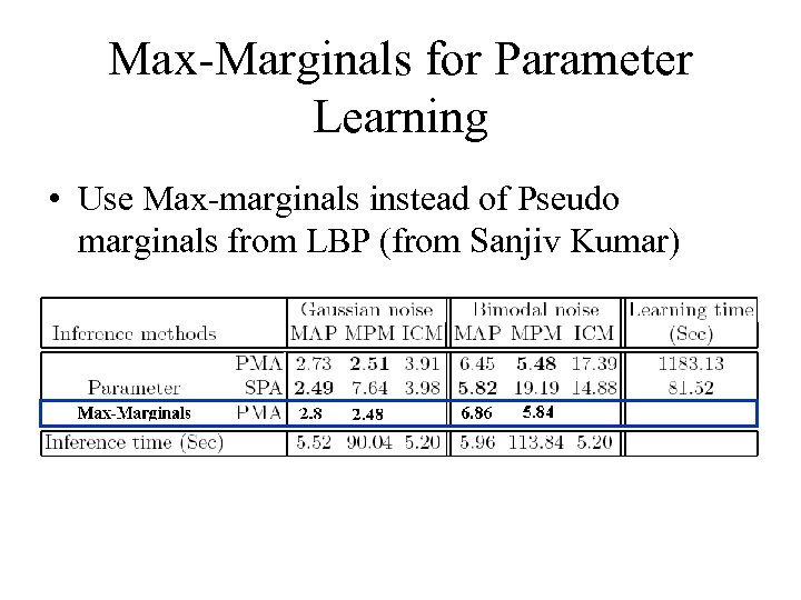
Max-Marginals for Parameter Learning • Use Max-marginals instead of Pseudo marginals from LBP (from Sanjiv Kumar)

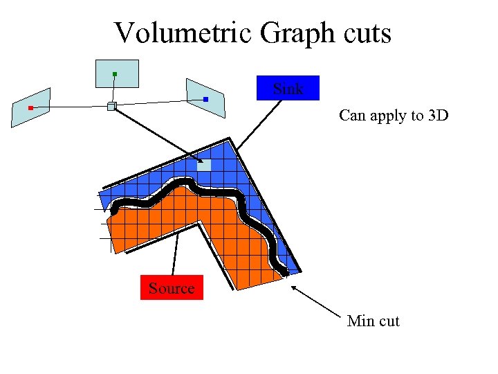
Volumetric Graph cuts Sink Can apply to 3 D Source Min cut

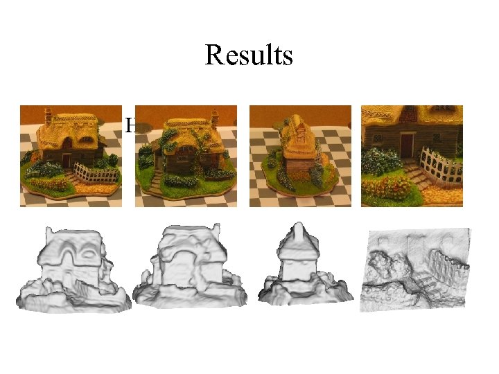
Results • Model House

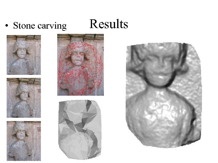
• Stone carving Results

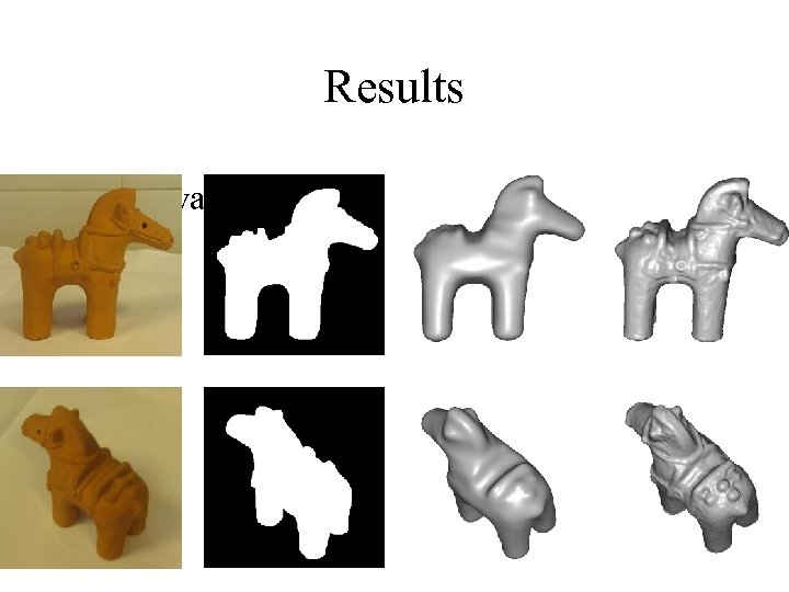
Results • Haniwa

Conclusion • Combining pose inference and segmentation worth investigating. • Lots more to do to extend MRF models • Combinatorial Optimization is a very interesting and hot area in vision at the moment. • Algorithms are as important as models.

Ask Pushmeet for code Demo