Coherent Measures of Risk in everyday market practice

Coherent Measures of Risk in everyday market practice Carlo Acerbi 4 th Annual CARISMA conference, London, July 2 2008

Motivations The present talk is a guided tour on the recent (sometimes very technical) literature on Coherent Measures of Risk (CMRs) Our purpose is to overview theory of coherent measures in the perspective of practical risk management applications. We will therefore focus on those results of theory which help understanding what coherent measures can today be considered as realistic candidate alternatives to Va. R in the market practice. This has also been the spirit of some research done in these years together with some collaborators of mine (Tasche, Simonetti)

Part 1: Coherency and Va. R shortcomings

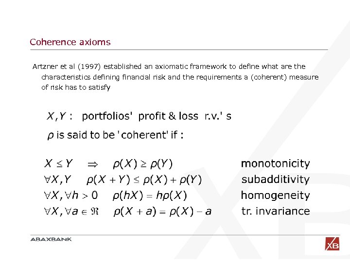Coherence axioms Artzner et al (1997) established an axiomatic framework to define what are the characteristics defining financial risk and the requirements a (coherent) measure of risk has to satisfy

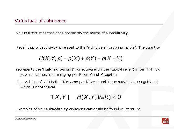Va. R’s lack of coherence Va. R is a statistics that does not satisfy the axiom of subadditivity. Recall that subadditivity is related to the “risk diversification principle”. The quantity represents the ‘hedging benefit’ (or equivalently the ‘capital relief’) in term of risk , which comes from merging portfolios X and Y together The problem of Va. R is that for some portfolios X and Y one may have a negative H, which is nonsensical Examples of Va. R subadditivity violations can easily be found in literature.

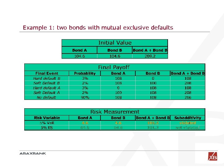Example 1: two bonds with mutual exclusive defaults

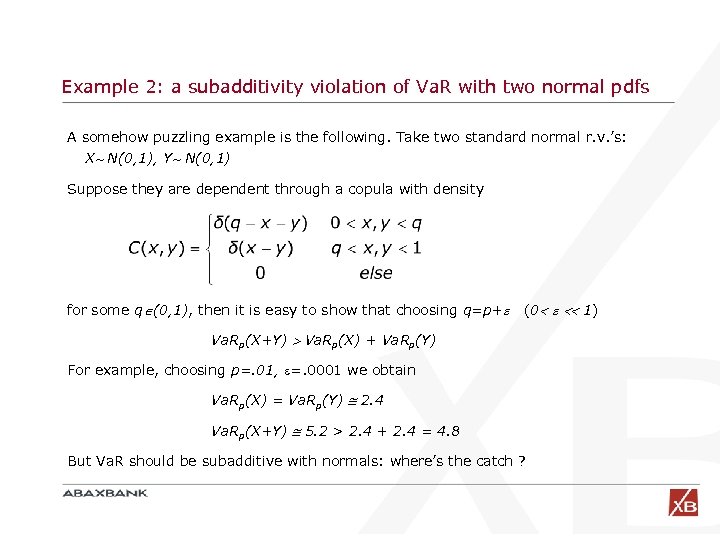Example 2: a subadditivity violation of Va. R with two normal pdfs A somehow puzzling example is the following. Take two standard normal r. v. ’s: X N(0, 1), Y N(0, 1) Suppose they are dependent through a copula with density for some q (0, 1), then it is easy to show that choosing q=p+ (0 1) Va. Rp(X+Y) Va. Rp(X) + Va. Rp(Y) For example, choosing p=. 01, =. 0001 we obtain Va. Rp(X) = Va. Rp(Y) 2. 4 Va. Rp(X+Y) 5. 2 > 2. 4 + 2. 4 = 4. 8 But Va. R should be subadditive with normals: where’s the catch ?

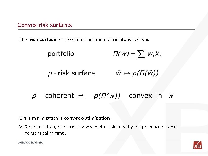Convex risk surfaces The ‘risk surface’ of a coherent risk measure is always convex. CRMs minimization is convex optimization. Va. R minimization, being not convex is often plagued by the presence of local nonsensical minima.

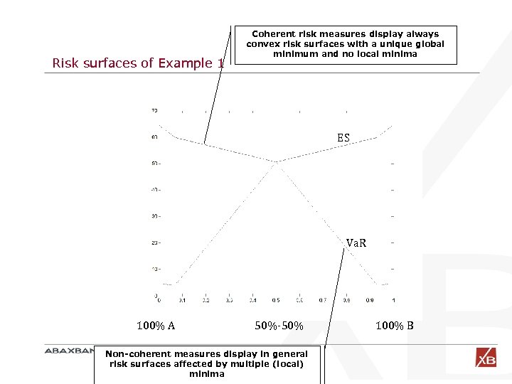Risk surfaces of Example 1 Coherent risk measures display always convex risk surfaces with a unique global minimum and no local minima ES Va. R 100% A 50%-50% Non-coherent measures display in general risk surfaces affected by multiple (local) minima 100% B

Example 3: a simple prototype portfolio Consider a portfolio made of n risky bonds all of which have a 3% default probability and suppose for simplicity that all the default probabilities are independent of one another. Portfolio = { 100 Euro invested in n i. i. d. Bonds } Bond payoff = Nominal (or 0 with probability 3%) Question: let’s choose n in such a way as to minimize the risk of the portfolio Let’s try to answer this question with a 5% Va. R, ES and TCE on a time horizon equal to the maturity of the bond.

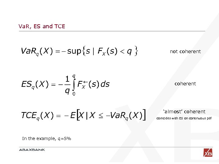Va. R, ES and TCE not coherent ‘almost’ coherent coincides with ES on continuous pdf In the example, q=5%

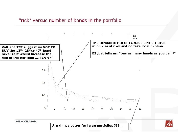“risk” versus number of bonds in the portfolio Va. R and TCE suggest us NOT TO BUY the 13 th, 28 thor 47 th bond because it would increase the risk of the portfolio. . (!? !? !? ) The surface of risk of ES has a single global minimum at n= and no fake local minima. ES just tells us: “buy as many bonds as you can !” Are things better for large portfolios ? ? ? . . .

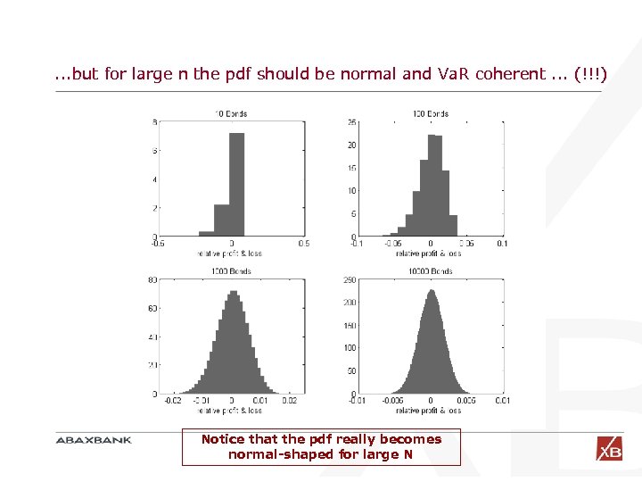. . . but for large n the pdf should be normal and Va. R coherent. . . (!!!) Notice that the pdf really becomes normal-shaped for large N

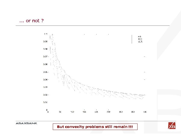. . . or not ? But convexity problems still remain !!!

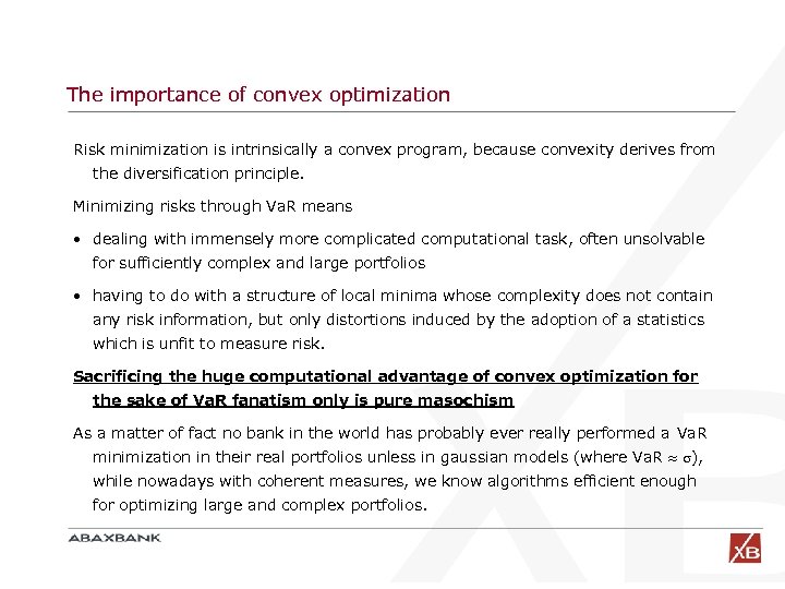The importance of convex optimization Risk minimization is intrinsically a convex program, because convexity derives from the diversification principle. Minimizing risks through Va. R means • dealing with immensely more complicated computational task, often unsolvable for sufficiently complex and large portfolios • having to do with a structure of local minima whose complexity does not contain any risk information, but only distortions induced by the adoption of a statistics which is unfit to measure risk. Sacrificing the huge computational advantage of convex optimization for the sake of Va. R fanatism only is pure masochism As a matter of fact no bank in the world has probably ever really performed a Va. R minimization in their real portfolios unless in gaussian models (where Va. R ), while nowadays with coherent measures, we know algorithms efficient enough for optimizing large and complex portfolios.

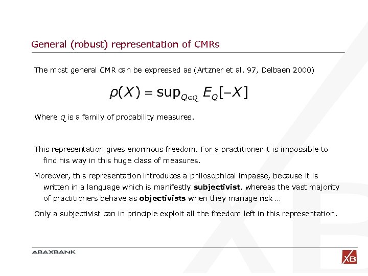General (robust) representation of CMRs The most general CMR can be expressed as (Artzner et al. 97, Delbaen 2000) Where Q is a family of probability measures. This representation gives enormous freedom. For a practitioner it is impossible to find his way in this huge class of measures. Moreover, this representation introduces a philosophical impasse, because it is written in a language which is manifestly subjectivist, whereas the vast majority of practitioners behave as objectivists when they manage risk … Only a subjectivist can in principle exploit all the freedom left in this representation.

The objectivist paradigm The main heritage of the advent of Va. R is probably the objectivist’s attitude a risk manager has learned to take 1. Model and fit the (real) probability distribution of your portfolio 2. Compute the quantile (Va. R) 3. Accepting this paradigm, we want to replace step 2 of this assembly line with suitable CMRs instead of Va. R 4. Notice that the (overwhelmingly larger) work done in the setup of 1 can be left as it is when replacing Va. R with any other measure. A change of paradigm (from obj. to subj. ) is very difficult to happen for the time being in risk mgmt practice.

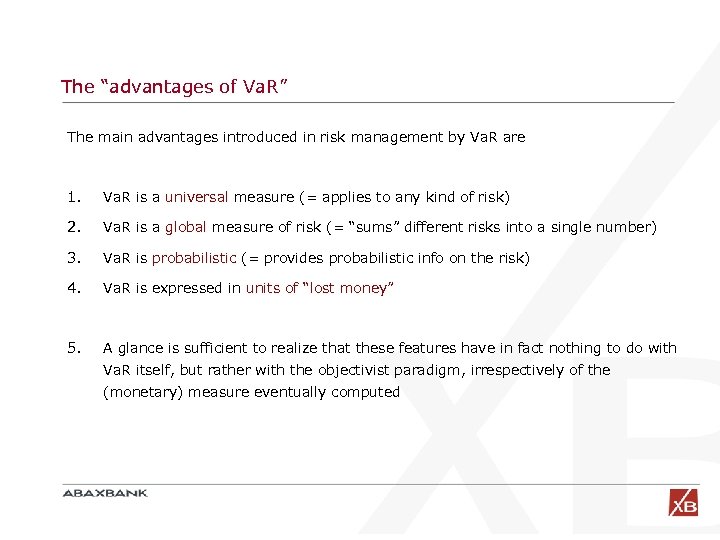The “advantages of Va. R” The main advantages introduced in risk management by Va. R are 1. Va. R is a universal measure (= applies to any kind of risk) 2. Va. R is a global measure of risk (= “sums” different risks into a single number) 3. Va. R is probabilistic (= provides probabilistic info on the risk) 4. Va. R is expressed in units of “lost money” 5. A glance is sufficient to realize that these features have in fact nothing to do with Va. R itself, but rather with the objectivist paradigm, irrespectively of the (monetary) measure eventually computed

Part 2: The importance of estimability

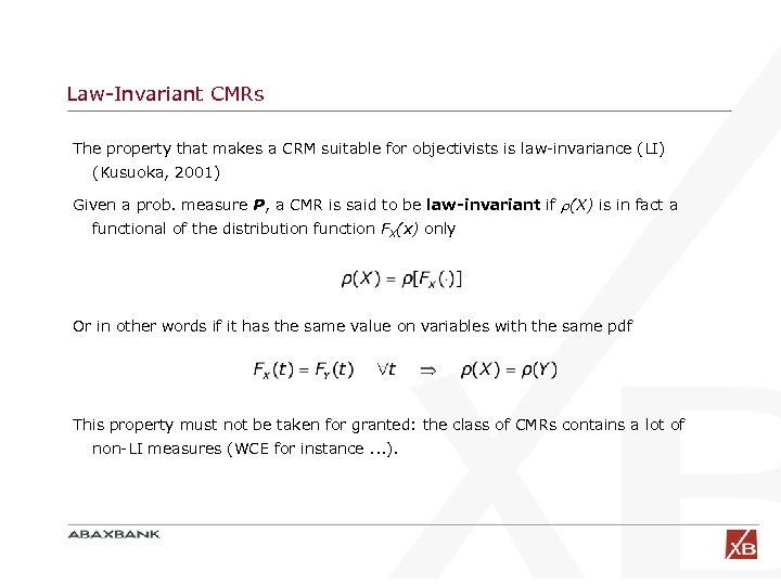Law-Invariant CMRs The property that makes a CRM suitable for objectivists is law-invariance (LI) (Kusuoka, 2001) Given a prob. measure P, a CMR is said to be law-invariant if (X) is in fact a functional of the distribution function FX(x) only Or in other words if it has the same value on variables with the same pdf This property must not be taken for granted: the class of CMRs contains a lot of non-LI measures (WCE for instance. . . ).

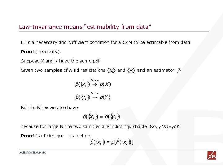Law-Invariance means “estimability from data” LI is a necessary and sufficient condition for a CRM to be estimable from data Proof (necessity): Suppose X and Y have the same pdf Given two samples of N iid realizations {xi} and {yi} and an estimator But for N we also have because for large N the two samples are indistinguishable. So, (X)= (Y) Proof (sufficiency): just define

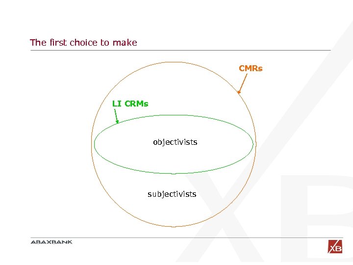The first choice to make CMRs LI CRMs objectivists subjectivists

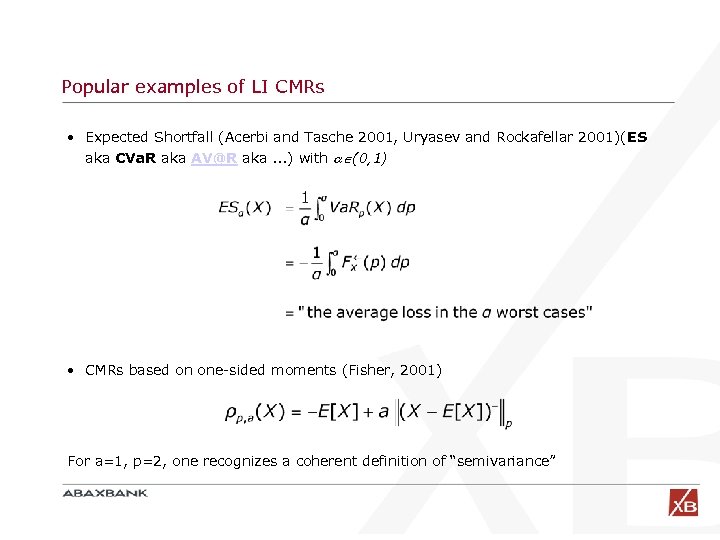Popular examples of LI CMRs • Expected Shortfall (Acerbi and Tasche 2001, Uryasev and Rockafellar 2001)(ES aka CVa. R aka AV@R aka. . . ) with (0, 1) • CMRs based on one-sided moments (Fisher, 2001) For a=1, p=2, one recognizes a coherent definition of “semivariance”

Part 3: Spectral Measures of Risk

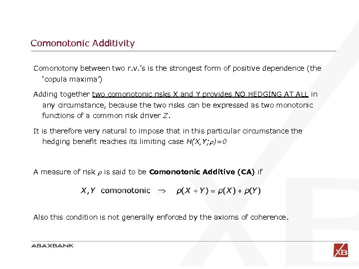Comonotonic Additivity Comonotony between two r. v. ’s is the strongest form of positive dependence (the ‘copula maxima’) Adding together two comonotonic risks X and Y provides NO HEDGING AT ALL in any circumstance, because the two risks can be expressed as two monotonic functions of a common risk driver Z. It is therefore very natural to impose that in this particular circumstance the hedging benefit reaches its limiting case H(X, Y; )=0 A measure of risk is said to be Comonotonic Additive (CA) if Also this condition is not generally enforced by the axioms of coherence.

Diversification principle revisited – cheating strategies In a context of capital adequacy the diversification principle is fully encoded in the couple of requirements 1. Subadditivity 2. Comonotonic Additivity (as a limiting case of subadditivity) To support this point of view it suffices to observe that if any of the two conditions is violated by a measure of risk used for capital adequacy, there exists a “cheating strategy” able to reduce the capital requirement without any real risk reduction. 1. “Split your portfolio into suitable subportfolios and compute capital adequacy on each one …” 2. “Merge your portfolio with the one of new ‘comonotone’ partners and compute capital adequacy on the global portfolio”

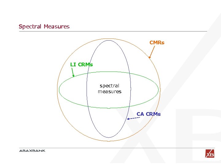
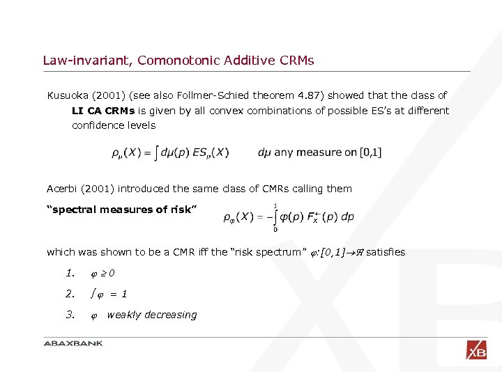Law-invariant, Comonotonic Additive CRMs Kusuoka (2001) (see also Follmer-Schied theorem 4. 87) showed that the class of LI CA CRMs is given by all convex combinations of possible ES’s at different confidence levels Acerbi (2001) introduced the same class of CMRs calling them “spectral measures of risk” which was shown to be a CMR iff the “risk spectrum” : [0, 1] satisfies 1. 0 2. =1 3. weakly decreasing

Law-invariant, Comonotonic Additive CRMs, (cont’d) It was soon realized that the class of LI CA CRMs = ‘Spectral Measures’ essentially coincided with the “distortion measures” dating back to the works of Denneberg (1990) and Wang (1996) in actuarial math, and in the context of premium principles (instead of coherence axioms)

Spectral Measures CMRs LI CRMs spectral measures CA CRMs

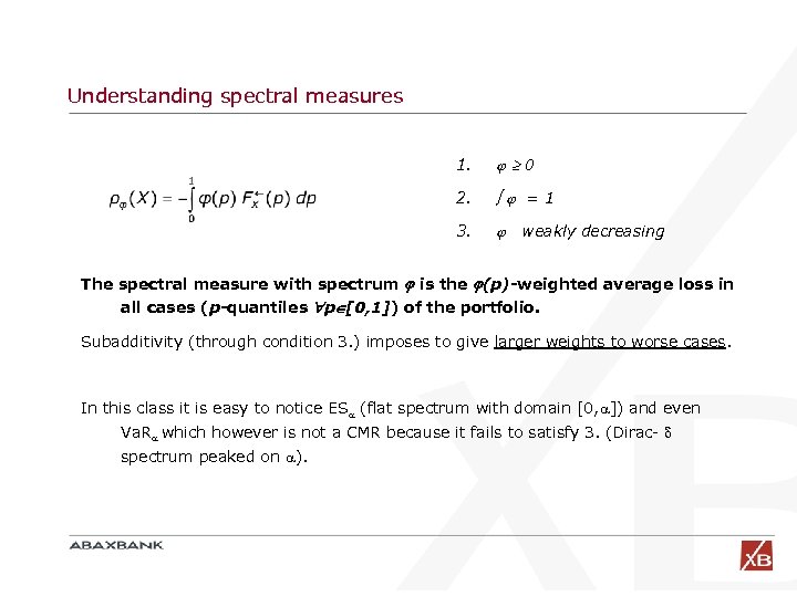Understanding spectral measures 1. 0 2. =1 3. weakly decreasing The spectral measure with spectrum is the (p)-weighted average loss in all cases (p-quantiles p [0, 1]) of the portfolio. Subadditivity (through condition 3. ) imposes to give larger weights to worse cases. In this class it is easy to notice ES (flat spectrum with domain [0, ]) and even Va. R which however is not a CMR because it fails to satisfy 3. (Dirac- spectrum peaked on ).

Part 4: Coherent Estimators

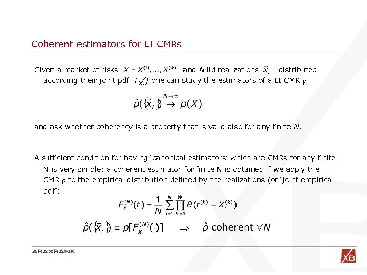Coherent estimators for LI CMRs Given a market of risks and N iid realizations distributed according their joint pdf FX() one can study the estimators of a LI CMR and ask whether coherency is a property that is valid also for any finite N. A sufficient condition for having ‘canonical estimators’ which are CMRs for any finite N is very simple: a coherent estimator finite N is obtained if we apply the CMR to the empirical distribution defined by the realizations (or ‘joint empirical pdf’)

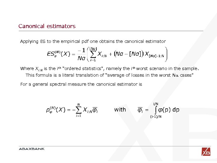Canonical estimators Applying ES to the empirical pdf one obtains the canonical estimator Where Xi: N is the ith “ordered statistics”, namely the ith worst scenario in the sample. This formula is a literal translation of “average of losses in the worst N cases” For a general spectral measure the canonical estimator is

Part 5: Optimization: exploiting convexity

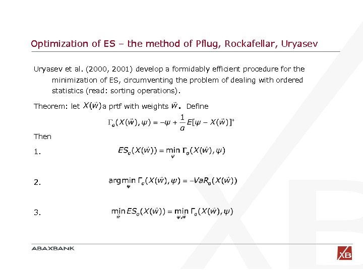Optimization of ES – the method of Pflug, Rockafellar, Uryasev et al. (2000, 2001) develop a formidably efficient procedure for the minimization of ES, circumventing the problem of dealing with ordered statistics (read: sorting operations). Theorem: let Then 1. 2. 3. a prtf with weights . Define

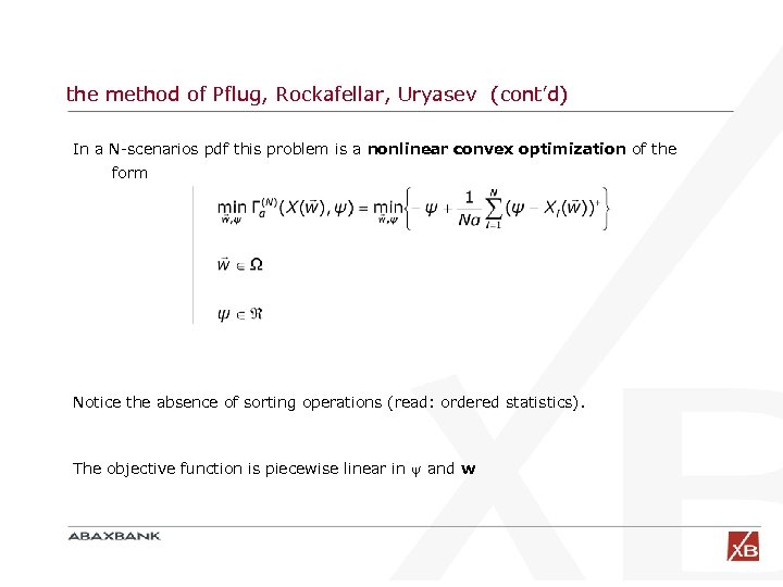the method of Pflug, Rockafellar, Uryasev (cont’d) In a N-scenarios pdf this problem is a nonlinear convex optimization of the form Notice the absence of sorting operations (read: ordered statistics). The objective function is piecewise linear in and w

the method of Pflug, Rockafellar, Uryasev (cont’d) But the problem can be mapped again into a linear optimization of the form Where linearity has been bought at the price of introducing n new variables z

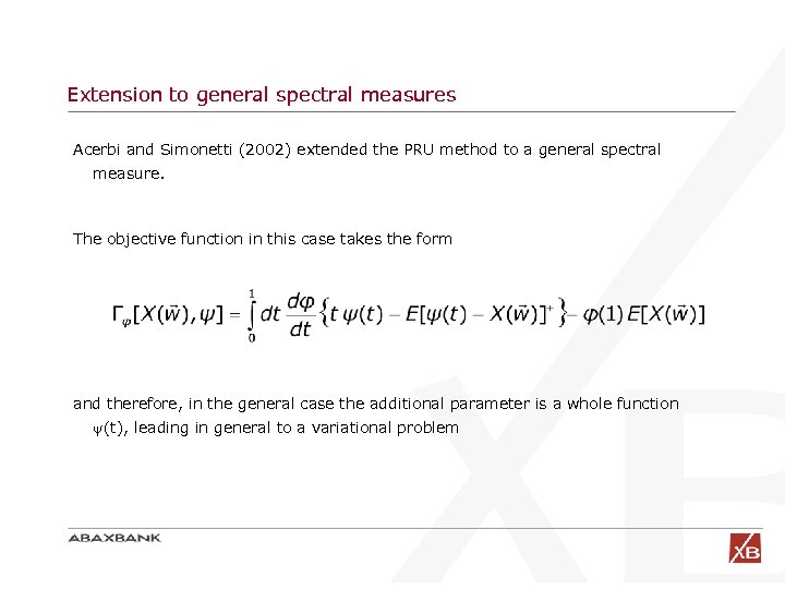Extension to general spectral measures Acerbi and Simonetti (2002) extended the PRU method to a general spectral measure. The objective function in this case takes the form and therefore, in the general case the additional parameter is a whole function (t), leading in general to a variational problem

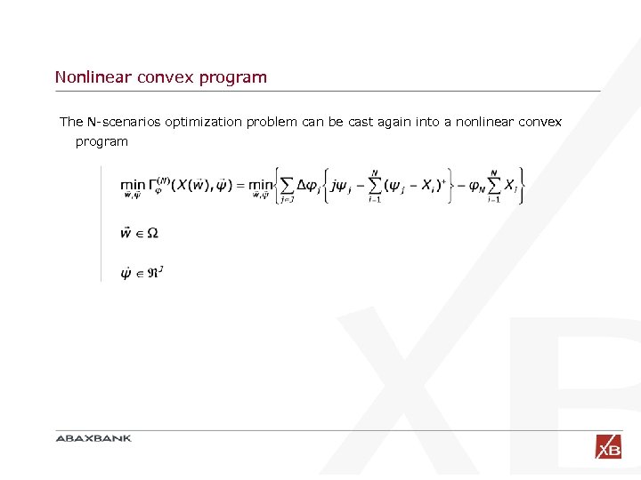Nonlinear convex program The N-scenarios optimization problem can be cast again into a nonlinear convex program

Linear program. . . or into a linear program in a (generally) huge number of variables

Conclusions The class of CMRs is too large. Unless an unlikely “subjectivistic revolution” takes place among risk practitioners, they will concentrate only on the Law-Invariant subclass All LI CRMs can replace Va. R in a risk management system, leaving unaltered most of it. They perfectly fit the objectivist paradigm and can share the same probabilistic hypotheses made for Va. R Among this subclass the further natural requirement of comonotonic additivity, identifies the family of ‘spectral measures of risk’ or ‘distorsion measures’. Spectral measures of risk, and in particular ES are gaining popularity because for these measures there exist consistent, coherent estimators and efficient convex optimization algorithms. As a matter of fact, optimization of large-complex portfolios is nowadays a realistic task to perform, under any probability measure modeling, within the class of spectral measures. Similar tasks were simply impossible with Va. R.

Suggested readings • Follmer and Schied: Stochastic Finance, 2 nd ed. , chapter 4 (2004) • Acerbi: “Coherent representations of subjective risk aversion”, in “Risk measures for the 21 st century”, (2004) And reference therein, in particular of the works of the following groups of researchers Artzner, Delbaen, Eber, Heath, Kusuoka Uryasev, Rockafellar, Pflug et al. Follmer, Schied, Acerbi, Tasche, Simonetti et al. Wang, Denneberg, et al Fisher others …