7d6645b65c63d3c5eb4f4ca849dd8a5b.ppt
- Количество слайдов: 88


Classification Michael I. Jordan University of California, Berkeley

Classification In classification problems, each entity in some domain can be placed in one of a discrete set of categories: yes/no, friend/foe, good/bad/indifferent, blue/red/green, etc. • Given a training set of labeled entities, develop a rule for assigning labels to entities in a test set • Many variations on this theme: • • • binary classification multi-category classification non-exclusive categories ranking Many criteria to assess rules and their predictions • • • overall errors costs associated with different kinds of errors operating points

Representation of Objects • Each object to be classified is represented as a pair (x, y): • • • where x is a description of the object (see examples of data types in the following slides) where y is a label (assumed binary for now) Success or failure of a machine learning classifier often depends on choosing good descriptions of objects • • the choice of description can also be viewed as a learning problem, and indeed we’ll discuss automated procedures for choosing descriptions in a later lecture but good human intuitions are often needed here

Data Types • Vectorial data: • • • physical attributes behavioral attributes context history etc We’ll assume for now that such vectors are explicitly represented in a table, but later (cf. kernel methods) we’ll relax that asumption

Data Types • text and hypertext <!DOCTYPE HTML PUBLIC "-//W 3 C//DTD HTML 4. 0 Transitional//EN"> <html> <head> <meta http-equiv="Content-Type" content="text/html; charset=utf-8"> <title>Welcome to Fairmont. NET</title> </head> <STYLE type="text/css">. stdtext {font-family: Verdana, Arial, Helvetica, sans-serif; font-size: 11 px; color: #1 F 3 D 4 E; }. stdtext_wh {font-family: Verdana, Arial, Helvetica, sans-serif; font-size: 11 px; color: WHITE; } </STYLE> <body leftmargin="0" topmargin="0" marginwidth="0" marginheight="0" bgcolor="BLACK" > <TABLE cellpadding="0" cellspacing="0" width="100%" border="0"> <TR> <TD width=50% background="/TFN/en/CDA/Images/common/labels/decorative_2 px_blk. gif"> </TD> <TD><img src="/TFN/en/CDA/Images/common/labels/decorative. gif"></td> <TD width=50% background="/TFN/en/CDA/Images/common/labels/decorative_2 px_blk. gif"> </TD> </TR> </TABLE> <tr> <td align="right" valign="middle"><IMG src="/TFN/en/CDA/Images/common/labels/centrino_logo_blk. gif"></td> </tr> </body> </html>

Data Types • email Return-path <bmiller@eecs. berkeley. edu>Received from relay 2. EECS. Berkeley. EDU (relay 2. EECS. Berkeley. EDU [169. 229. 60. 28]) by imap 4. CS. Berkeley. EDU (i. Planet Messaging Server 5. 2 Hot. Fix 1. 16 (built May 14 2003)) with ESMTP id <0 HZ 000 F 506 JV 5 S@imap 4. CS. Berkeley. EDU>; Tue, 08 Jun 2004 11: 40: 43 -0700 (PDT)Received from relay 3. EECS. Berkeley. EDU (localhost [127. 0. 0. 1]) by relay 2. EECS. Berkeley. EDU (8. 12. 10/8. 9. 3) with ESMTP id i 58 Ieg 3 N 000927; Tue, 08 Jun 2004 11: 40: 43 -0700 (PDT)Received from redbirds (dhcp-168 -35. EECS. Berkeley. EDU [128. 32. 168. 35]) by relay 3. EECS. Berkeley. EDU (8. 12. 10/8. 9. 3) with ESMTP id i 58 Ieg. Fp 007613; Tue, 08 Jun 2004 11: 40: 42 -0700 (PDT)Date Tue, 08 Jun 2004 11: 40: 42 -0700 From Robert Miller <bmiller@eecs. berkeley. edu>Subject RE: SLT headcount = 25 In-replyto <6. 1. 1. 1. 0. 20040607101523. 02623298@imap. eecs. Berkeley. edu>To 'Randy Katz' <randy@eecs. berkeley. edu>Cc "'Glenda J. Smith'" <glendajs@eecs. berkeley. edu>, 'Gert Lanckriet' <gert@eecs. berkeley. edu>Messageid <200406081840. i 58 Ieg. Fp 007613@relay 3. EECS. Berkeley. EDU>MIME-version 1. 0 XMIMEOLE Produced By Microsoft Mime. OLE V 6. 00. 2800. 1409 X-Mailer Microsoft Office Outlook, Build 11. 0. 5510 Content-type multipart/alternative; boundary="---=_Next. Part_000_0033_01 C 44 D 4 D. 6 DD 93 AF 0"Threadindex Ac. RMt. QRp+R 26 l. VFa. Riuz 4 Bf. Imik. TRAA 0 wf 3 Qthe headcount is now 32. -------------------- Robert Miller, Administrative Specialist University of California, Berkeley Electronics Research Lab 634 Soda Hall #1776 Berkeley, CA 94720 -1776 Phone: 510 -642 -6037 fax: 510 -643 -1289

Data Types • protein sequences

Data Types • sequences of Unix system calls

Data Types • network layout: graph

Data Types • images

Example: Spam Filter • • • Input: email Output: spam/ham Setup: • • Get a large collection of example emails, each labeled “spam” or “ham” Note: someone has to hand label all this data Want to learn to predict labels of new, future emails Features: The attributes used to make the ham / spam decision • • Words: FREE! Text Patterns: $dd, CAPS Non-text: Sender. In. Contacts … Dear Sir. First, I must solicit your confidence in this transaction, this is by virture of its nature as being utterly confidencial and top secret. … TO BE REMOVED FROM FUTURE MAILINGS, SIMPLY REPLY TO THIS MESSAGE AND PUT "REMOVE" IN THE SUBJECT. 99 MILLION EMAIL ADDRESSES FOR ONLY $99 Ok, Iknow this is blatantly OT but I'm beginning to go insane. Had an old Dell Dimension XPS sitting in the corner and decided to put it to use, I know it was working pre being stuck in the corner, but when I plugged it in, hit the power nothing happened.

Example: Digit Recognition • • • Input: images / pixel grids Output: a digit 0 -9 Setup: • • • Get a large collection of example images, each labeled with a digit Note: someone has to hand label all this data Want to learn to predict labels of new, future digit images 0 1 2 Features: The attributes used to make the digit decision • Pixels: (6, 8)=ON • Shape Patterns: Num. Components, Aspect. Ratio, Num. Loops • … Current state-of-the-art: Human-level performance 1 ? ?

Other Examples of Real-World Classification Tasks • • • Fraud detection (input: account activity, classes: fraud / no fraud) Web page spam detection (input: HTML/rendered page, classes: spam / ham) Speech recognition and speaker recognition (input: waveform, classes: phonemes or words) Medical diagnosis (input: symptoms, classes: diseases) Automatic essay grader (input: document, classes: grades) Customer service email routing and foldering Link prediction in social networks Catalytic activity in drug design … many more • Classification is an important commercial technology • • •

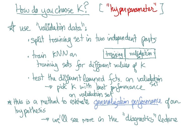
Training and Validation • Data: labeled instances, e. g. emails marked spam/ham • • Training • • • Estimate parameters on training set Tune hyperparameters on validation set Report results on test set Anything short of this yields over-optimistic claims Training Data Evaluation • • • Training set Validation set Test set Many different metrics Ideally, the criteria used to train the classifier should be closely related to those used to evaluate the classifier Statistical issues • • • Want a classifier which does well on test data Overfitting: fitting the training data very closely, but not generalizing well Error bars: want realistic (conservative) estimates of accuracy Validation Data Test Data

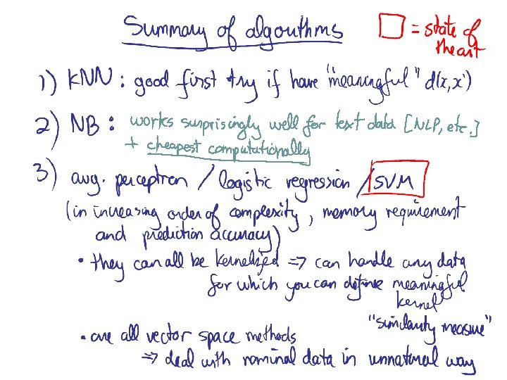
Some State-of-the-art Classifiers • • Support vector machine Random forests Kernelized logistic regression Kernelized discriminant analysis Kernelized perceptron Bayesian classifiers Boosting and other ensemble methods (Nearest neighbor)

Intuitive Picture of the Problem Class 1 Class 2

Some Issues • • • There may be a simple separator (e. g. , a straight line in 2 D or a hyperplane in general) or there may not There may be “noise” of various kinds There may be “overlap” One should not be deceived by one’s low-dimensional geometrical intuition Some classifiers explicitly represent separators (e. g. , straight lines), while for other classifiers the separation is done implicitly Some classifiers just make a decision as to which class an object is in; others estimate class probabilities
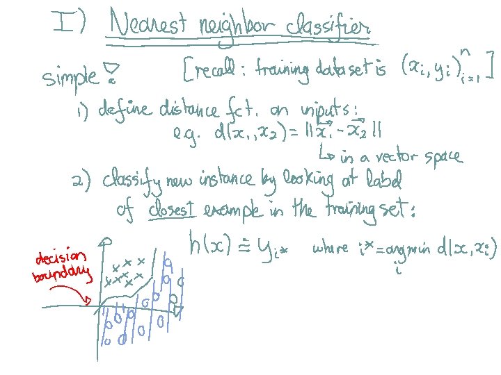
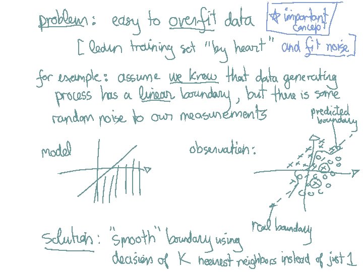
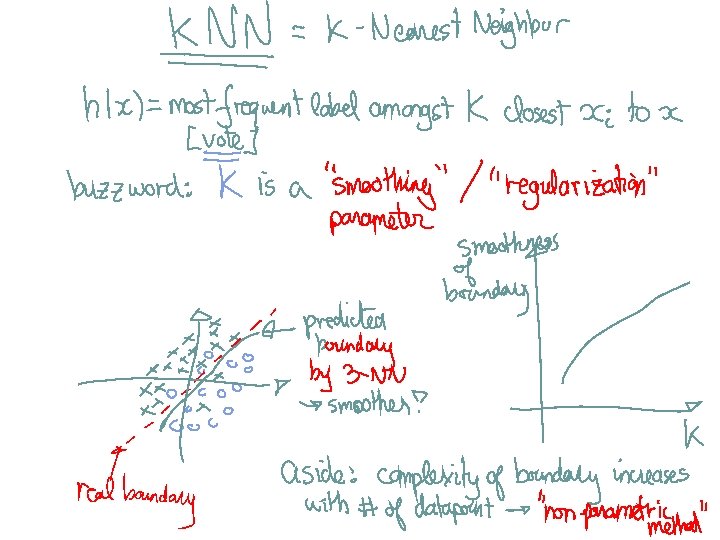
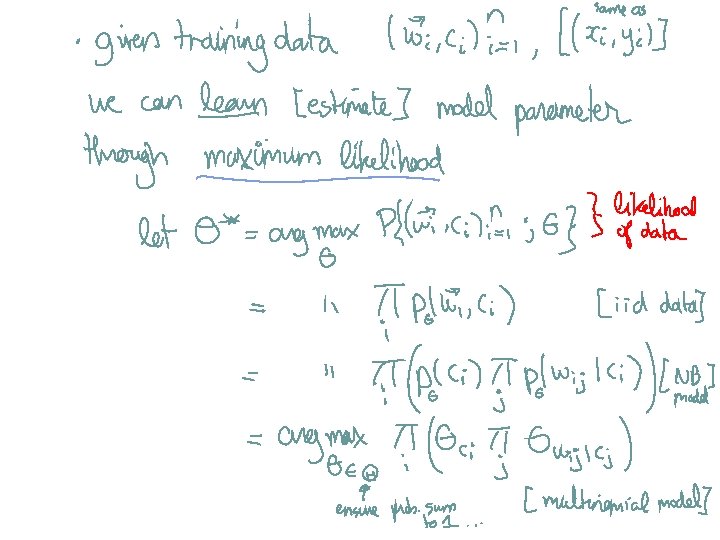
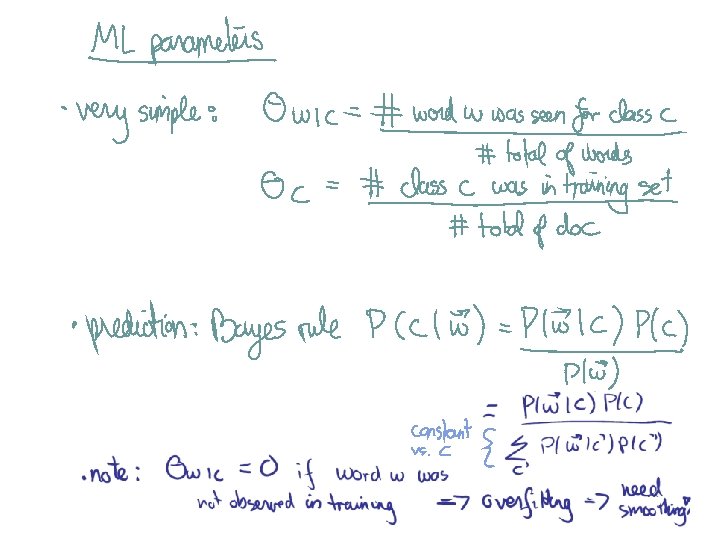
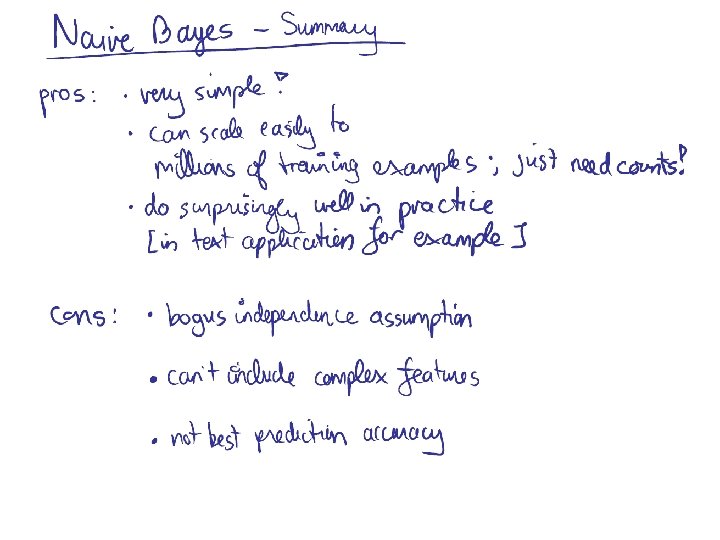
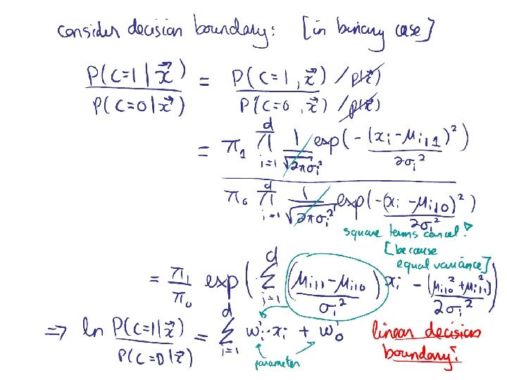
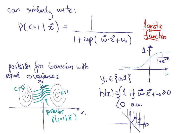
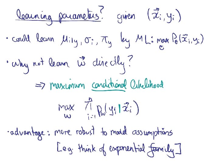
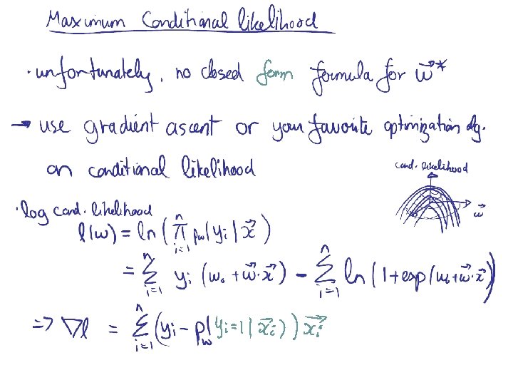
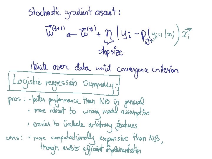
 Instance-based methods: 1) Nearest neighbor II) Probabilistic models: 1) Naïve Bayes 2)")
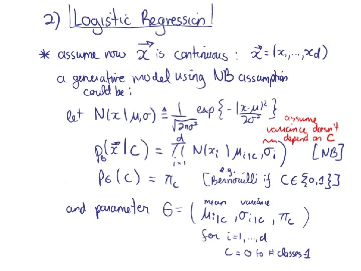
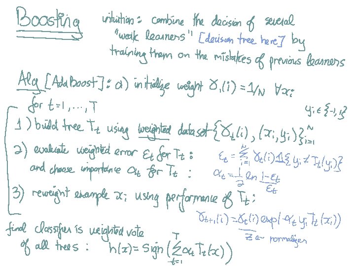
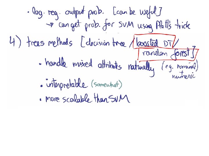
Methods I) Instance-based methods: 1) Nearest neighbor II) Probabilistic models: 1) Naïve Bayes 2) Logistic Regression III) Linear Models: 1) Perceptron 2) Support Vector Machine IV) Decision Models: 1) Decision Trees 2) Boosted Decision Trees 3) Random Forest
 Instance-based methods: 1) Nearest neighbor II) Probabilistic models: 1) Naïve Bayes 2)")
Methods I) Instance-based methods: 1) Nearest neighbor II) Probabilistic models: 1) Naïve Bayes 2) Logistic Regression III) Linear Models: 1) Perceptron 2) Support Vector Machine IV) Decision Models: 1) Decision Trees 2) Boosted Decision Trees 3) Random Forest

Linearly Separable Data Linear Decision boundary Class 1 Class 2

Nonlinearly Separable Data Non Linear Classifier Class 1 Class 2

Which Separating Hyperplane to Use? x 1 x 2

Maximizing the Margin x 1 Select the separating hyperplane that maximizes the margin Margin Width x 2

Support Vectors x 1 Support Vectors Margin Width x 2

Setting Up the Optimization Problem x 1 The maximum margin can be characterized as a solution to an optimization problem: x 2

Setting Up the Optimization Problem • If class 1 corresponds to 1 and class 2 corresponds to -1, we can rewrite • as • So the problem becomes: or

Linear, Hard-Margin SVM Formulation • Find w, b that solves Problem is convex so, there is a unique global minimum value (when feasible) • There is also a unique minimizer, i. e. weight and b value that provides the minimum • Quadratic Programming • very efficient computationally with procedures that take advantage of the special structure •

Nonlinearly Separable Data Var 1 Introduce slack variables Allow some instances to fall within the margin, but penalize them Var 2

Formulating the Optimization Problem Constraints becomes : Var 1 Objective function penalizes for misclassified instances and those within the margin Var 2 C trades-off margin width and misclassifications

Linear, Soft-Margin SVMs Algorithm tries to maintain i to zero while maximizing margin • Notice: algorithm does not minimize the number of misclassifications (NP-complete problem) but the sum of distances from the margin hyperplanes • Other formulations use i 2 instead • As C 0, we get the hard-margin solution •

Robustness of Soft vs Hard Margin SVMs Var 1 i Var 2 Soft Margin SVN Hard Margin SVN

Disadvantages of Linear Decision Surfaces Var 1 Var 2

Advantages of Nonlinear Surfaces Var 1 Var 2

Linear Classifiers in High. Dimensional Spaces Var 1 Constructed Feature 2 Var 2 Find function (x) to map to a different space Constructed Feature 1
 to map to")
Mapping Data to a High. Dimensional Space • Find function (x) to map to a different space, then SVM formulation becomes: • Data appear as (x), weights w are now weights in the new space • Explicit mapping expensive if (x) is very high dimensional • Solving the problem without explicitly mapping the data is desirable
")
The Dual of the SVM Formulation • Original SVM formulation • • The (Wolfe) dual of this problem • • • n inequality constraints n positivity constraints n number of variables one equality constraint n positivity constraints n number of variables (Lagrange multipliers) Objective function more complicated NOTE: Data only appear as (xi) (xj)
 (xj): means, map data into new space, then take the")
The Kernel Trick (xi) (xj): means, map data into new space, then take the inner product of the new vectors • We can find a function such that: K(xi xj) = (xi) (xj), i. e. , the image of the inner product of the data is the inner product of the images of the data • Then, we do not need to explicitly map the data into the highdimensional space to solve the optimization problem •
![Example w. T (x)+b=0 X=[x z] (X)=[x 2 z 2 xz] f(x) = sign(w](https://present5.com/presentation/7d6645b65c63d3c5eb4f4ca849dd8a5b/image-60.jpg "Example w. T (x)+b=0 X=[x z] (X)=[x 2 z 2 xz] f(x) = sign(w")
Example w. T (x)+b=0 X=[x z] (X)=[x 2 z 2 xz] f(x) = sign(w 1 x 2+w 2 z 2+w 3 xz + b)
![Example X 1=[x 1 z 1] X 2=[x 2 z 2] (X 1)=[x 12](https://present5.com/presentation/7d6645b65c63d3c5eb4f4ca849dd8a5b/image-61.jpg "Example X 1=[x 1 z 1] X 2=[x 2 z 2] (X 1)=[x 12")
Example X 1=[x 1 z 1] X 2=[x 2 z 2] (X 1)=[x 12 z 12 21/2 x 1 z 1] (X 2)=[x 22 z 22 21/2 x 2 z 2] (X 1)T (X 2)= [x 12 z 12 21/2 x 1 z 1] [x 22 z 22 21/2 x 2 z 2]T Expensive! = x 12 z 12 + x 22 z 22 + 2 x 1 z 1 x 2 O(d 2) z 2 = (x 1 z 1 + x 2 z 2)2 = (X 1 T X 2)2 Efficient! O(d)

Kernel Trick Kernel function: a symmetric function k : Rd x Rd -> R • Inner product kernels: additionally, k(x, z) = (x)T (z) • Example: • O(d 2) O(d)

Kernel Trick Implement an infinite-dimensional mapping implicitly • Only inner products explicitly needed for training and evaluation • Inner products computed efficiently, in finite dimensions • The underlying mathematical theory is that of reproducing kernel Hilbert space from functional analysis •

Kernel Methods • If a linear algorithm can be expressed only in terms of inner products • • it can be “kernelized” find linear pattern in high-dimensional space nonlinear relation in original space Specific kernel function determines nonlinearity
 = x.")
Kernels • Some simple kernels • • • Linear kernel: k(x, z) = x. Tz equivalent to linear algorithm Polynomial kernel: k(x, z) = (1+x. Tz)d polynomial decision rules RBF kernel: k(x, z) = exp(-||x-z||2/2 ) highly nonlinear decisions

Gaussian Kernel: Example A hyperplane in some space
 • • • Kernel matrix K defines all pairwise inner")
Kernel Matrix k(x, y) • • • Kernel matrix K defines all pairwise inner products Mercer theorem: K positive semidefinite Any symmetric positive semidefinite matrix can be regarded as an inner product matrix in some space i K j Kij=k(xi, xj)
} • k(x, y) or • y")
Kernel-Based Learning Data Embedding Linear algorithm {(xi, yi)} • k(x, y) or • y K

Kernel-Based Learning Data Embedding Linear algorithm K Kernel design Kernel algorithm

Kernel Design Simple kernels on vector data • More advanced • • • string kernel diffusion kernels over general structures (sets, trees, graphs. . . ) kernels derived from graphical models empirical kernel map
 Instance-based methods: 1) Nearest neighbor II) Probabilistic models: 1) Naïve Bayes 2)")
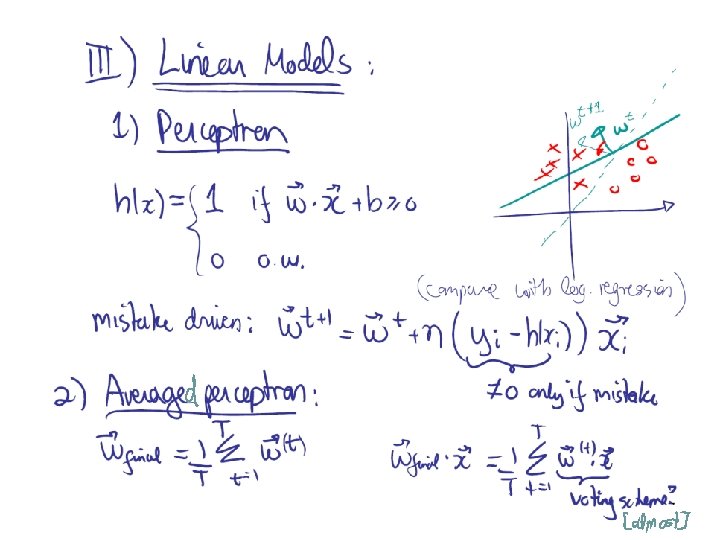
Methods I) Instance-based methods: 1) Nearest neighbor II) Probabilistic models: 1) Naïve Bayes 2) Logistic Regression III) Linear Models: 1) Perceptron 2) Support Vector Machine IV) Decision Models: 1) Decision Trees 2) Boosted Decision Trees 3) Random Forest
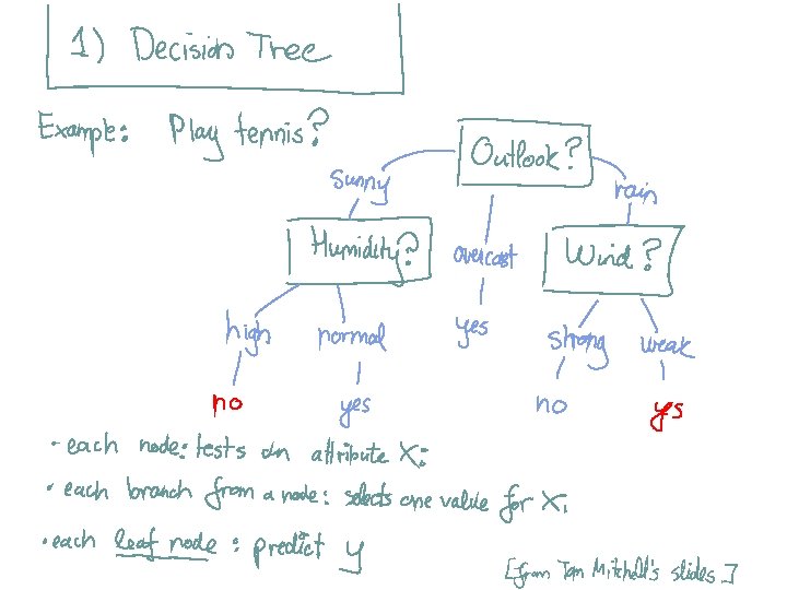
![[From Tom Mitchell’s slides]](https://present5.com/presentation/7d6645b65c63d3c5eb4f4ca849dd8a5b/image-73.jpg "[From Tom Mitchell’s slides]")
[From Tom Mitchell’s slides]

Spatial example: recursive binary splits + + ++ + + +

Spatial example: recursive binary splits + + ++ + + +

Spatial example: recursive binary splits + + ++ + + +

Spatial example: recursive binary splits + + ++ + + +

Spatial example: recursive binary splits + + ++ + + + Once regions are chosen class probabilities are easy to calculate pm=5/6
 • Information")
How to choose a split N 1=9 p 1=8/9 Impurity measures: L(p) • Information gain (entropy): - p log p - (1 -p) log(1 -p) • Gini index: 2 p (1 -p) + + C 1 ++ + + + C 2 p 2=5/6 N 2=6 • ( 0 -1 error: 1 -max(p, 1 -p) ) s min N 1 L(p 1)+N 2 L(p 2) s Then choose the region that has the best split

Overfitting and pruning L: 0 -1 loss + + + + + min. T åi L(xi) + |T| then choose with CV increase a + +
 Instance-based methods: 1) Nearest neighbor II) Probabilistic models: 1) Naïve Bayes 2)")
Methods I) Instance-based methods: 1) Nearest neighbor II) Probabilistic models: 1) Naïve Bayes 2) Logistic Regression III) Linear Models: 1) Perceptron 2) Support Vector Machine IV) Decision Models: 1) Decision Trees 2) Boosted Decision Trees 3) Random Forest

Random Forest Randomly sample 2/3 of the data Data Each node: pick randomly a small m number of input variables to split on VOTE ! Use Out-Of-Bag samples to: - Estimate error - Choosing m - Estimate variable importance
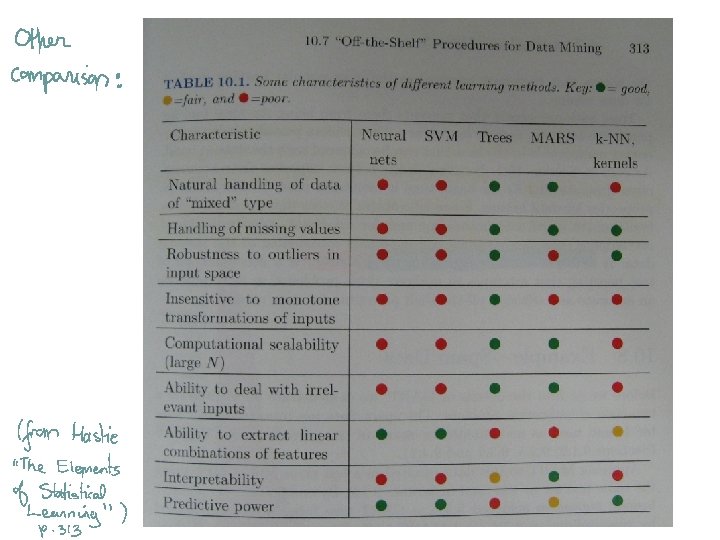

Reading • All of the methods that we have discussed are presented in the following book: Hastie, T. , Tibshirani, R. & Friedman, J. (2009). The Elements of Statistical Learning: Data Mining, Inference, and Prediction (Second Edition), NY: Springer. • We haven’t discussed theory, but if you’re interested in theory of (binary) classification, here’s a pointer to get started: Bartlett, P. , Jordan, M. I. , & Mc. Auliffe, J. D. (2006). Convexity, classification and risk bounds. Journal of the American Statistical Association, 101, 138 -156.
7d6645b65c63d3c5eb4f4ca849dd8a5b.ppt