b078260d12411335c259818c201145a6.ppt
- Количество слайдов: 25
 Classification and Regression
 Classification and regression What is classification? What is regression? p Issues regarding classification and regression p Classification by decision tree induction p Bayesian Classification p Other Classification Methods p regression p
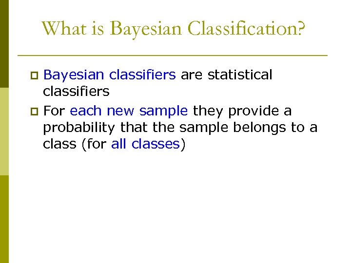 What is Bayesian Classification? Bayesian classifiers are statistical classifiers p For each new sample they provide a probability that the sample belongs to a class (for all classes) p
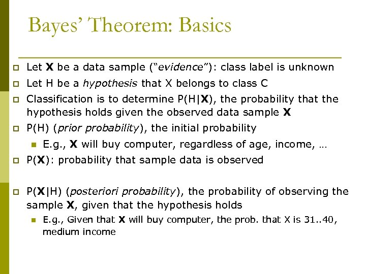 Bayes’ Theorem: Basics p Let X be a data sample (“evidence”): class label is unknown p Let H be a hypothesis that X belongs to class C p Classification is to determine P(H|X), the probability that the hypothesis holds given the observed data sample X p P(H) (prior probability), the initial probability n E. g. , X will buy computer, regardless of age, income, … p P(X): probability that sample data is observed p P(X|H) (posteriori probability), the probability of observing the sample X, given that the hypothesis holds n E. g. , Given that X will buy computer, the prob. that X is 31. . 40, medium income
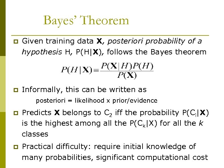 Bayes’ Theorem p Given training data X, posteriori probability of a hypothesis H, P(H|X), follows the Bayes theorem p Informally, this can be written as posteriori = likelihood x prior/evidence p Predicts X belongs to C 2 iff the probability P(Ci|X) is the highest among all the P(Ck|X) for all the k classes p Practical difficulty: require initial knowledge of many probabilities, significant computational cost
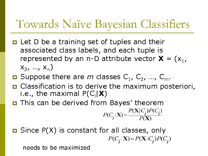 Towards Naïve Bayesian Classifiers p Let D be a training set of tuples and their associated class labels, and each tuple is represented by an n-D attribute vector X = (x 1, x 2, …, xn) Suppose there are m classes C 1, C 2, …, Cm. Classification is to derive the maximum posteriori, i. e. , the maximal P(Ci|X) This can be derived from Bayes’ theorem p Since P(X) is constant for all classes, only p p p needs to be maximized
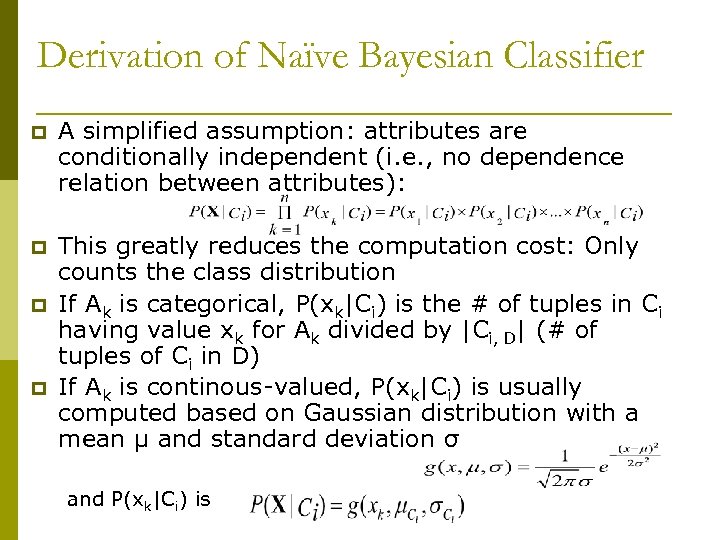 Derivation of Naïve Bayesian Classifier p A simplified assumption: attributes are conditionally independent (i. e. , no dependence relation between attributes): p This greatly reduces the computation cost: Only counts the class distribution If Ak is categorical, P(xk|Ci) is the # of tuples in Ci having value xk for Ak divided by |Ci, D| (# of tuples of Ci in D) If Ak is continous-valued, P(xk|Ci) is usually computed based on Gaussian distribution with a mean μ and standard deviation σ p p and P(xk|Ci) is
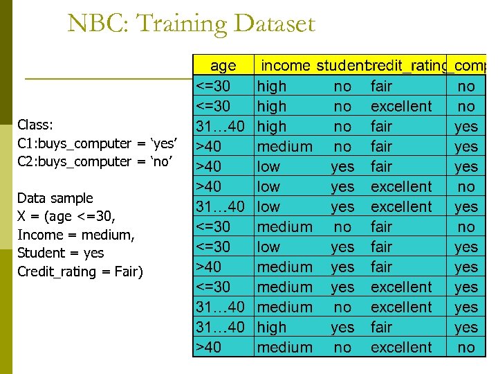 NBC: Training Dataset Class: C 1: buys_computer = ‘yes’ C 2: buys_computer = ‘no’ Data sample X = (age <=30, Income = medium, Student = yes Credit_rating = Fair)
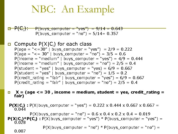 NBC: An Example p P(Ci): p Compute P(X|Ci) for each class P(buys_computer = “yes”) = 9/14 = 0. 643 P(buys_computer = “no”) = 5/14= 0. 357 P(age = “<=30” | buys_computer = “yes”) = 2/9 = 0. 222 P(age = “<= 30” | buys_computer = “no”) = 3/5 = 0. 6 P(income = “medium” | buys_computer = “yes”) = 4/9 = 0. 444 P(income = “medium” | buys_computer = “no”) = 2/5 = 0. 4 P(student = “yes” | buys_computer = “yes) = 6/9 = 0. 667 P(student = “yes” | buys_computer = “no”) = 1/5 = 0. 2 P(credit_rating = “fair” | buys_computer = “yes”) = 6/9 = 0. 667 P(credit_rating = “fair” | buys_computer = “no”) = 2/5 = 0. 4 p X = (age <= 30 , income = medium, student = yes, credit_rating = fair) P(X|Ci) : P(X|buys_computer = “yes”) = 0. 222 x 0. 444 x 0. 667 = 0. 044 P(X|buys_computer = “no”) = 0. 6 x 0. 4 x 0. 2 x 0. 4 = 0. 019 P(X|Ci)*P(Ci) : P(X|buys_computer = “yes”) * P(buys_computer = “yes”) = 0. 028 P(X|buys_computer = “no”) * P(buys_computer = “no”) = 0. 007
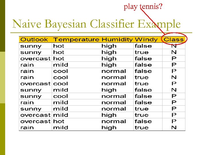 play tennis? Naive Bayesian Classifier Example
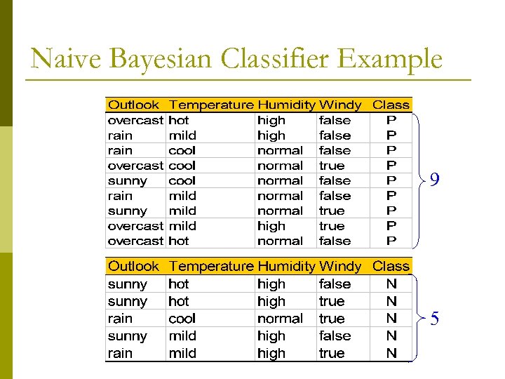 Naive Bayesian Classifier Example 9 5
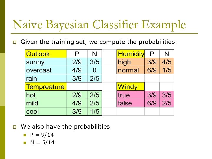 Naive Bayesian Classifier Example p Given the training set, we compute the probabilities: p We also have the probabilities n n P = 9/14 N = 5/14
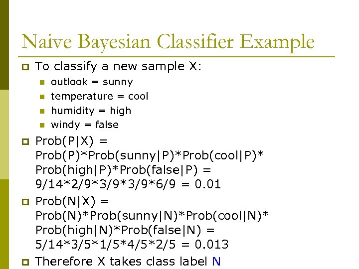 Naive Bayesian Classifier Example p To classify a new sample X: n n p p p outlook = sunny temperature = cool humidity = high windy = false Prob(P|X) = Prob(P)*Prob(sunny|P)*Prob(cool|P)* Prob(high|P)*Prob(false|P) = 9/14*2/9*3/9*6/9 = 0. 01 Prob(N|X) = Prob(N)*Prob(sunny|N)*Prob(cool|N)* Prob(high|N)*Prob(false|N) = 5/14*3/5*1/5*4/5*2/5 = 0. 013 Therefore X takes class label N
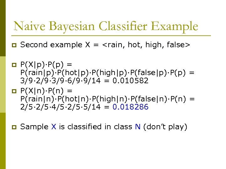 Naive Bayesian Classifier Example p Second example X =
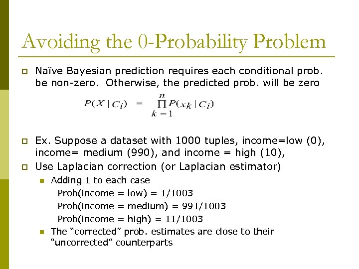 Avoiding the 0 -Probability Problem p Naïve Bayesian prediction requires each conditional prob. be non-zero. Otherwise, the predicted prob. will be zero p Ex. Suppose a dataset with 1000 tuples, income=low (0), income= medium (990), and income = high (10), Use Laplacian correction (or Laplacian estimator) p n n Adding 1 to each case Prob(income = low) = 1/1003 Prob(income = medium) = 991/1003 Prob(income = high) = 11/1003 The “corrected” prob. estimates are close to their “uncorrected” counterparts
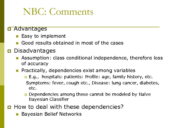 NBC: Comments p Advantages n n p Easy to implement Good results obtained in most of the cases Disadvantages n n Assumption: class conditional independence, therefore loss of accuracy Practically, dependencies exist among variables E. g. , hospitals: patients: Profile: age, family history, etc. Symptoms: fever, cough etc. , Disease: lung cancer, diabetes, etc. p Dependencies among these cannot be modeled by Naïve Bayesian Classifier p p How to deal with these dependencies? n Bayesian Belief Networks
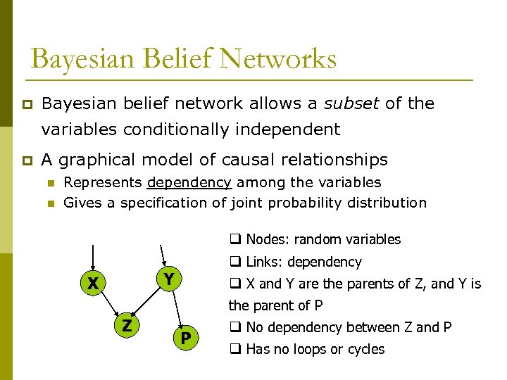 Bayesian Belief Networks p Bayesian belief network allows a subset of the variables conditionally independent p A graphical model of causal relationships n n Represents dependency among the variables Gives a specification of joint probability distribution q Nodes: random variables q Links: dependency Y X q X and Y are the parents of Z, and Y is the parent of P Z P q No dependency between Z and P q Has no loops or cycles
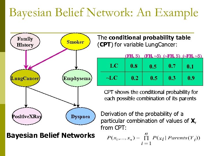 Bayesian Belief Network: An Example Family History Smoker The conditional probability table (CPT) for variable Lung. Cancer: (FH, S) (FH, ~S) (~FH, ~S) LC Lung. Cancer Emphysema 0. 8 0. 5 0. 7 0. 1 ~LC 0. 2 0. 5 0. 3 0. 9 CPT shows the conditional probability for each possible combination of its parents Positive. XRay Dyspnea Bayesian Belief Networks Derivation of the probability of a particular combination of values of X, from CPT:
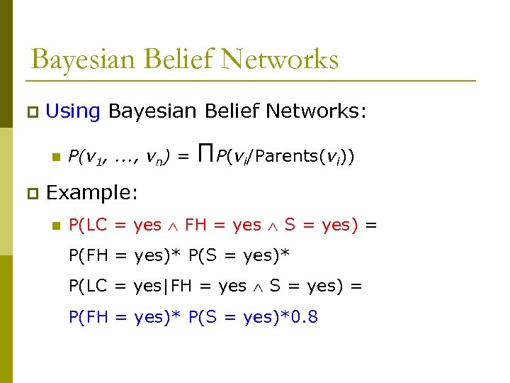 Bayesian Belief Networks p Using Bayesian Belief Networks: n p P(v 1, . . . , vn) = ΠP(vi/Parents(vi)) Example: n P(LC = yes FH = yes S = yes) = P(FH = yes)* P(S = yes)* P(LC = yes|FH = yes S = yes) = P(FH = yes)* P(S = yes)*0. 8
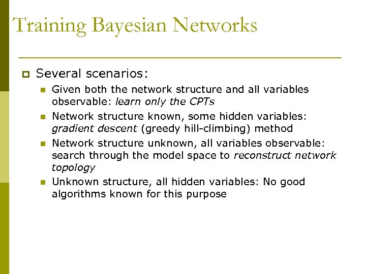 Training Bayesian Networks p Several scenarios: n n Given both the network structure and all variables observable: learn only the CPTs Network structure known, some hidden variables: gradient descent (greedy hill-climbing) method Network structure unknown, all variables observable: search through the model space to reconstruct network topology Unknown structure, all hidden variables: No good algorithms known for this purpose
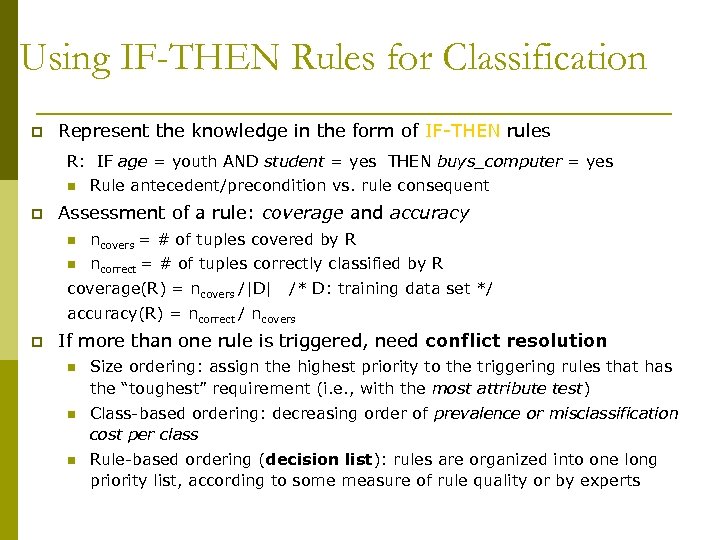 Using IF-THEN Rules for Classification p Represent the knowledge in the form of IF-THEN rules R: IF age = youth AND student = yes THEN buys_computer = yes n p Rule antecedent/precondition vs. rule consequent Assessment of a rule: coverage and accuracy n ncovers = # of tuples covered by R n ncorrect = # of tuples correctly classified by R coverage(R) = ncovers /|D| /* D: training data set */ accuracy(R) = ncorrect / ncovers p If more than one rule is triggered, need conflict resolution n Size ordering: assign the highest priority to the triggering rules that has the “toughest” requirement (i. e. , with the most attribute test) n Class-based ordering: decreasing order of prevalence or misclassification cost per class n Rule-based ordering (decision list): rules are organized into one long priority list, according to some measure of rule quality or by experts
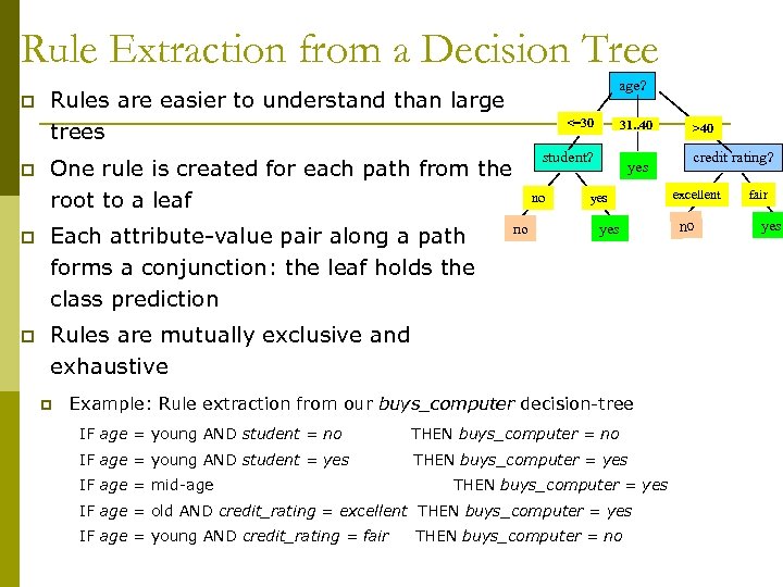 Rule Extraction from a Decision Tree p p age? Rules are easier to understand than large trees <=30 student? One rule is created for each path from the root to a leaf p Each attribute-value pair along a path forms a conjunction: the leaf holds the class prediction p 31. . 40 no no yes yes Rules are mutually exclusive and exhaustive p Example: Rule extraction from our buys_computer decision-tree IF age = young AND student = no THEN buys_computer = no IF age = young AND student = yes THEN buys_computer = yes IF age = mid-age THEN buys_computer = yes IF age = old AND credit_rating = excellent THEN buys_computer = yes IF age = young AND credit_rating = fair THEN buys_computer = no >40 credit rating? excellent no fair yes
 Instance-Based Methods p Instance-based learning: n p Store training examples and delay the processing (“lazy evaluation”) until a new instance must be classified Typical approaches n k-nearest neighbor approach p Instances represented as points in a Euclidean space.
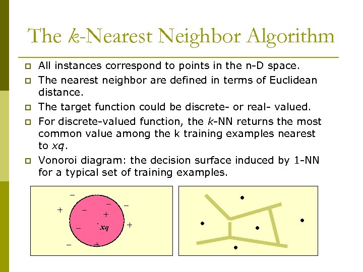 The k-Nearest Neighbor Algorithm p p p All instances correspond to points in the n-D space. The nearest neighbor are defined in terms of Euclidean distance. The target function could be discrete- or real- valued. For discrete-valued function, the k-NN returns the most common value among the k training examples nearest to xq. Vonoroi diagram: the decision surface induced by 1 -NN for a typical set of training examples. _ _ _ + _ _ . + + xq . _ + . .
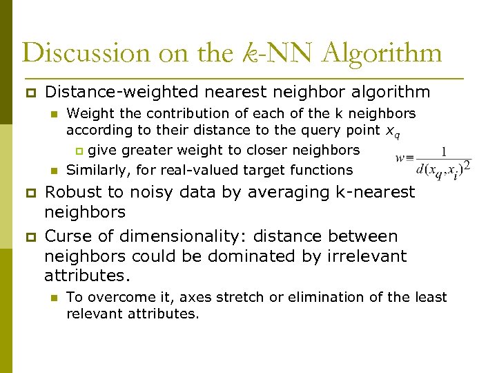 Discussion on the k-NN Algorithm p Distance-weighted nearest neighbor algorithm n n p p Weight the contribution of each of the k neighbors according to their distance to the query point xq p give greater weight to closer neighbors Similarly, for real-valued target functions Robust to noisy data by averaging k-nearest neighbors Curse of dimensionality: distance between neighbors could be dominated by irrelevant attributes. n To overcome it, axes stretch or elimination of the least relevant attributes.


