Class Forecasting techniques for RM 1 Naïve approach

Class Forecasting techniques for RM 1. Naïve approach 2. Qualitative methods (EJM) 3. Decision making methods under uncertainty 4. Quantitative methods: - Moving averages (SMA, WMA, EMA) - Linear regression Seasonality (2 techniques) Study materials: Slides RM, v. 3/2011, A. Zaporozhetz 1

Forecasting (Greek: pro + gnosis) - projecting future financial or operational information (e. g. , sales, expenses, quantities sold, etc. ); - a prediction of future events or conditions; - the process of estimation in unknown situations. (SMA 2 A) Forecasting support systems – software with forecasting functions: Statistica, SPSS, Forecast. Pro, Mat. Lab, Stat. Pad… Based on math methods (regression models, moving averages). They will NOT do the job for you RM, v. 3/2011, A. Zaporozhetz 2

Risk and Forecasting “Risk - the chance that an outcome will be different than expected; can be measured as the degree of variability in either an individual’s or an organization’s anticipated investment outcomes. ” (SMA 2 A) Q: How can we manage risks with effective forecasting? RM, v. 3/2011, A. Zaporozhetz 3

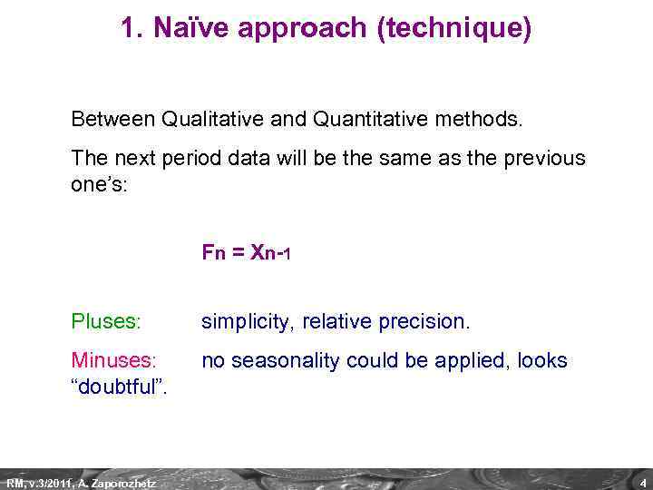1. Naïve approach (technique) Between Qualitative and Quantitative methods. The next period data will be the same as the previous one’s: F n = X n -1 Pluses: simplicity, relative precision. Minuses: “doubtful”. no seasonality could be applied, looks RM, v. 3/2011, A. Zaporozhetz 4

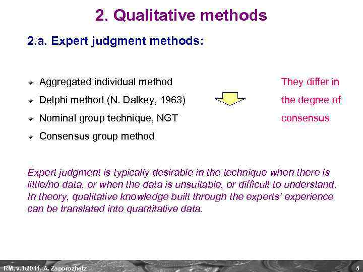2. Qualitative methods 2. a. Expert judgment methods: Aggregated individual method They differ in Delphi method (N. Dalkey, 1963) the degree of Nominal group technique, NGT consensus Consensus group method Expert judgment is typically desirable in the technique when there is little/no data, or when the data is unsuitable, or difficult to understand. In theory, qualitative knowledge built through the experts’ experience can be translated into quantitative data. RM, v. 3/2011, A. Zaporozhetz 5

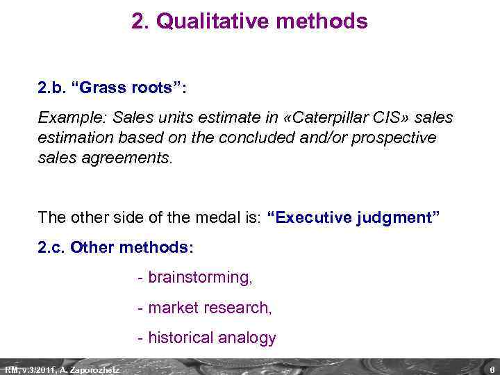2. Qualitative methods 2. b. “Grass roots”: Example: Sales units estimate in «Caterpillar CIS» sales estimation based on the concluded and/or prospective sales agreements. The other side of the medal is: “Executive judgment” 2. c. Other methods: - brainstorming, - market research, - historical analogy RM, v. 3/2011, A. Zaporozhetz 6

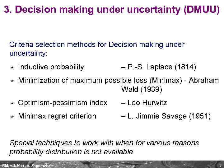3. Decision making under uncertainty (DMUU) Criteria selection methods for Decision making under uncertainty: Inductive probability – P. -S. Laplace (1814) Minimization of maximum possible loss (Minimax) - Abraham Wald (1939) Optimism-pessimism index – Leo Hurwitz Minimax regret criterion – L. Jimmie Savage (1951) Special techniques to work with when for various reasons probability distribution is not available. RM, v. 3/2011, A. Zaporozhetz 7

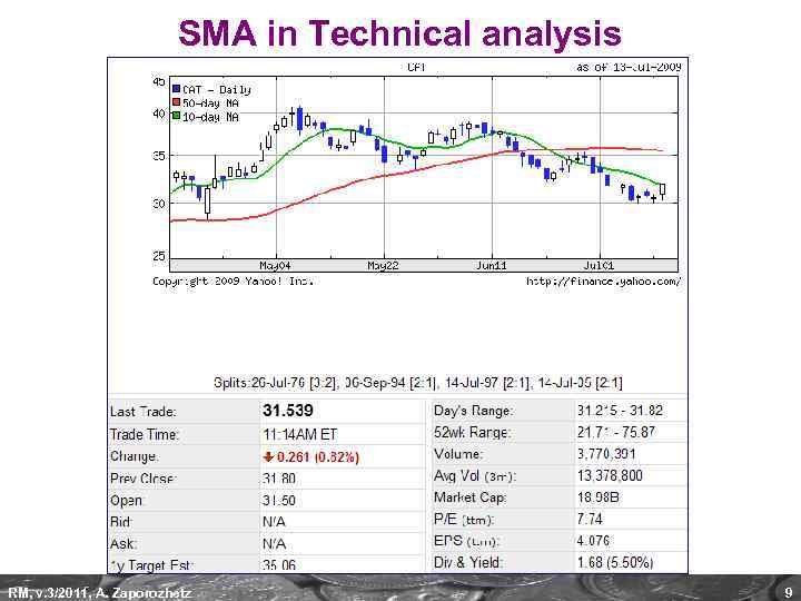
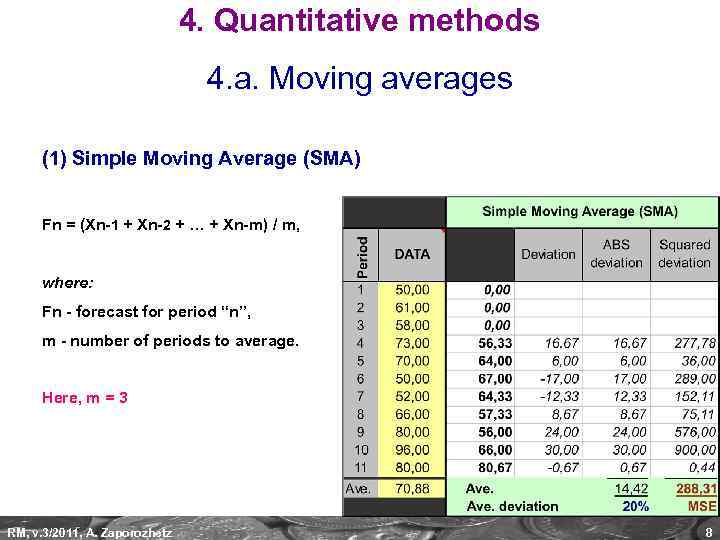4. Quantitative methods 4. a. Moving averages (1) Simple Moving Average (SMA) Fn = (Xn-1 + Xn-2 + … + Xn-m) / m, where: Fn - forecast for period “n”, m - number of periods to average. Here, m = 3 RM, v. 3/2011, A. Zaporozhetz 8

SMA in Technical analysis RM, v. 3/2011, A. Zaporozhetz 9

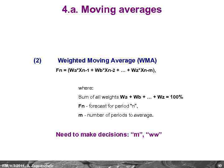4. a. Moving averages (2) Weighted Moving Average (WMA) Fn = (Wa*Xn-1 + Wb*Xn-2 + … + Wz*Xn-m), where: Sum of all weights Wa + Wb + … + Wz = 100% Fn - forecast for period “n”, m - number of periods to average. Need to make decisions: “m”, “ww” RM, v. 3/2011, A. Zaporozhetz 10

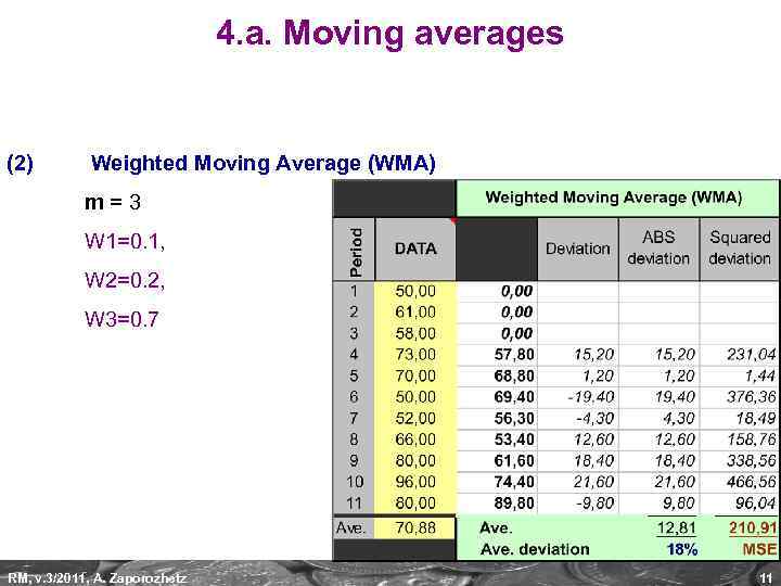4. a. Moving averages (2) Weighted Moving Average (WMA) m=3 W 1=0. 1, W 2=0. 2, W 3=0. 7 RM, v. 3/2011, A. Zaporozhetz 11

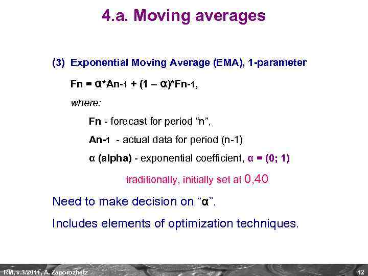4. a. Moving averages (3) Exponential Moving Average (EMA), 1 -parameter Fn = α*An-1 + (1 – α)*Fn-1, where: Fn - forecast for period “n”, An-1 - actual data for period (n-1) α (alpha) - exponential coefficient, α = (0; 1) traditionally, initially set at 0, 40 Need to make decision on “α”. Includes elements of optimization techniques. RM, v. 3/2011, A. Zaporozhetz 12

4. a. Moving averages (3) Exponential Moving Average (EMA), 1 -parameter Fn = α*An-1 + (1 – α)*Fn-1 can also be expressed as: Fn = Fn-1 + α*(An-1 - Fn-1). We see that if alpha approaches 1, then Fn would tend to the value of An-1. If Fn is equal to An-1, then we face the naïve model. RM, v. 3/2011, A. Zaporozhetz 13

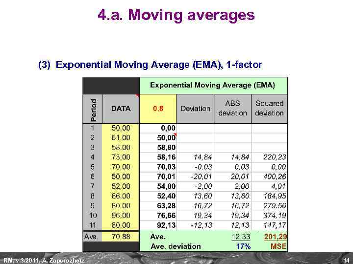4. a. Moving averages (3) Exponential Moving Average (EMA), 1 -factor RM, v. 3/2011, A. Zaporozhetz 14

4. a. Moving averages Pluses: Minuses: RM, v. 3/2011, A. Zaporozhetz simplicity. difficult to apply seasonality, only 1 next period can be forecasted. 15

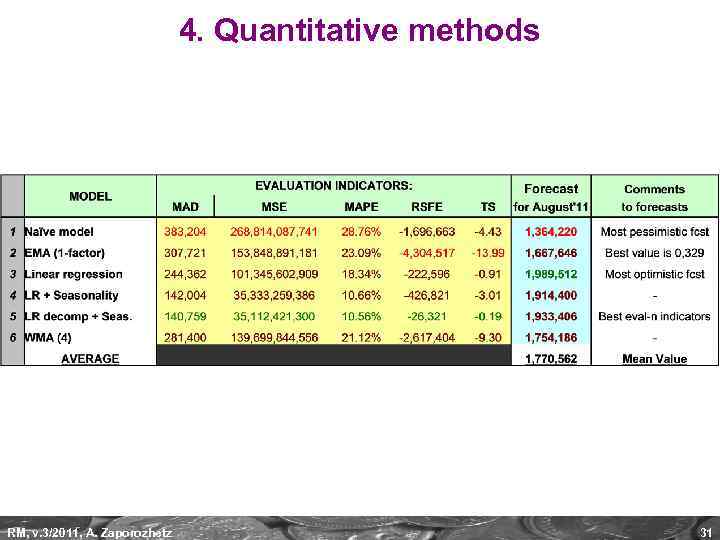
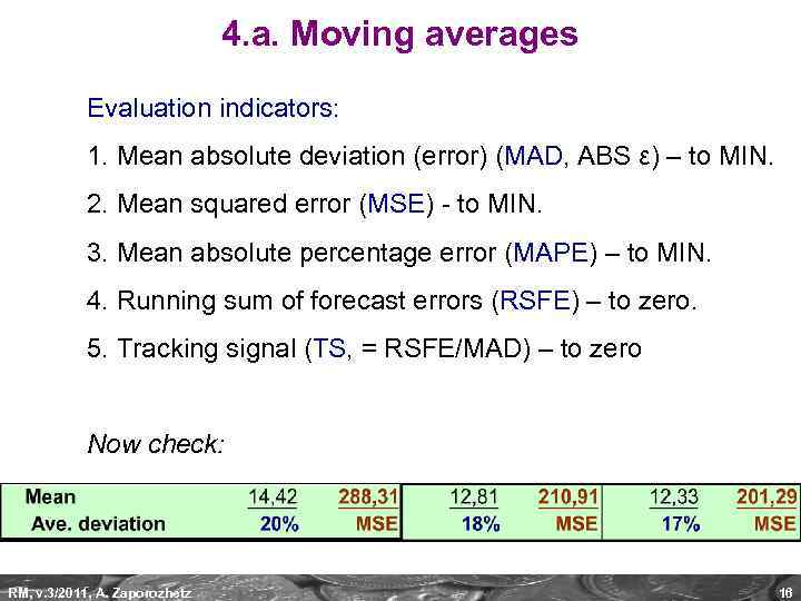4. a. Moving averages Evaluation indicators: 1. Mean absolute deviation (error) (MAD, ABS ε) – to MIN. 2. Mean squared error (MSE) - to MIN. 3. Mean absolute percentage error (MAPE) – to MIN. 4. Running sum of forecast errors (RSFE) – to zero. 5. Tracking signal (TS, = RSFE/MAD) – to zero Now check: RM, v. 3/2011, A. Zaporozhetz 16

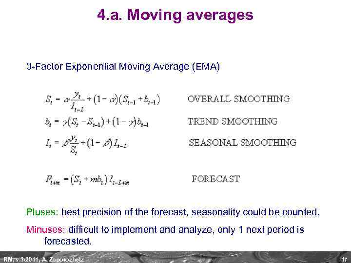4. a. Moving averages 3 -Factor Exponential Moving Average (EMA) Pluses: best precision of the forecast, seasonality could be counted. Minuses: difficult to implement and analyze, only 1 next period is forecasted. RM, v. 3/2011, A. Zaporozhetz 17

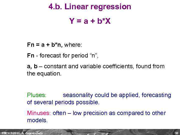4. b. Linear regression Y = a + b*X Fn = a + b*n, where: Fn - forecast for period “n”, a, b – constant and variable coefficients, found from the equation. Pluses: seasonality could be applied, forecasting of several periods possible. Minuses: often – low precision as compared to other models. RM, v. 3/2011, A. Zaporozhetz 18

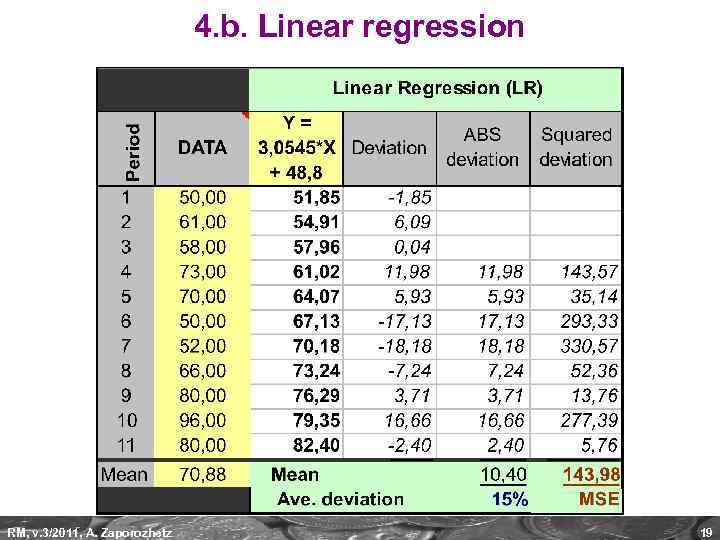4. b. Linear regression RM, v. 3/2011, A. Zaporozhetz 19

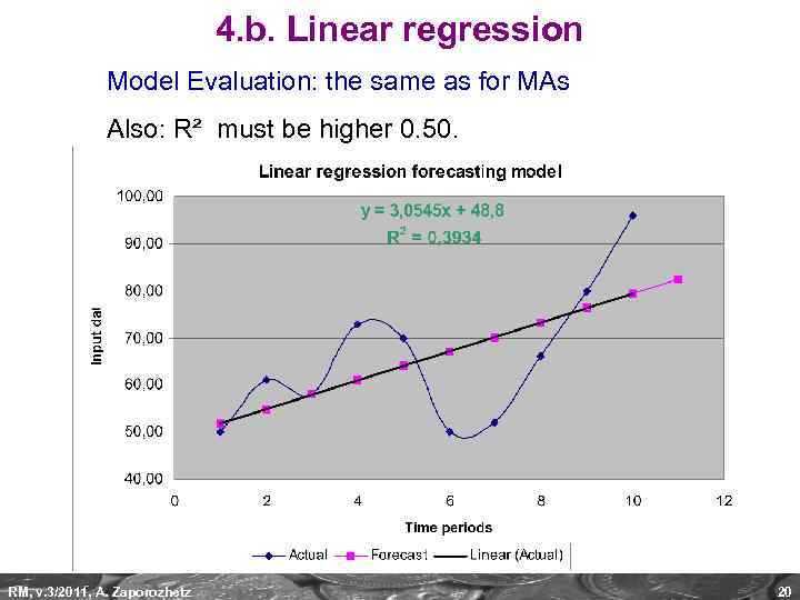4. b. Linear regression Model Evaluation: the same as for MAs Also: R² must be higher 0. 50. RM, v. 3/2011, A. Zaporozhetz 20

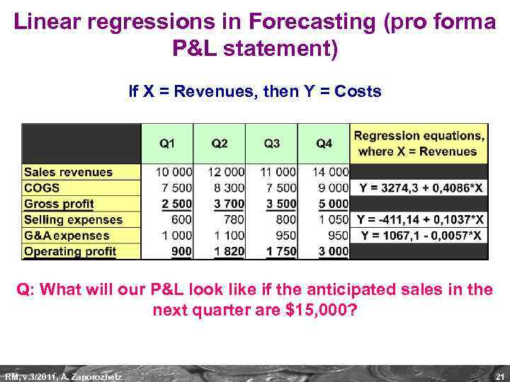Linear regressions in Forecasting (pro forma P&L statement) If X = Revenues, then Y = Costs Q: What will our P&L look like if the anticipated sales in the next quarter are $15, 000? RM, v. 3/2011, A. Zaporozhetz 21

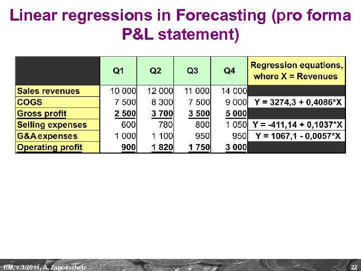Linear regressions in Forecasting (pro forma P&L statement) RM, v. 3/2011, A. Zaporozhetz 22

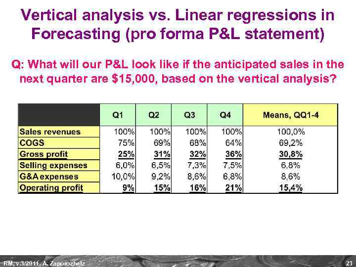Vertical analysis vs. Linear regressions in Forecasting (pro forma P&L statement) Q: What will our P&L look like if the anticipated sales in the next quarter are $15, 000, based on the vertical analysis? RM, v. 3/2011, A. Zaporozhetz 23

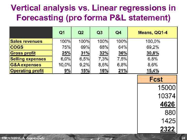Vertical analysis vs. Linear regressions in Forecasting (pro forma P&L statement) RM, v. 3/2011, A. Zaporozhetz 24

Vertical analysis vs. Linear regressions in Forecasting (pro forma P&L statement) Which one do you think is more realistic? RM, v. 3/2011, A. Zaporozhetz 25

Seasonality – observed periodic and regular changes of input time series data depending on: ►season, quarter, ►month, week, day of the week, ►particular date (holiday, etc). Necessary data: at least TWO recurring periods E. g. , 8 quarters, 24 months, etc. RM, v. 3/2011, A. Zaporozhetz 26

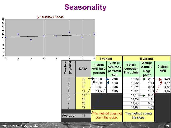Seasonality RM, v. 3/2011, A. Zaporozhetz 27

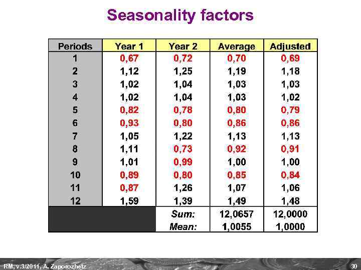
Seasonality factors Finding out seasonality factors presence: no less than 75% of periods observed. E. g. , in at least 6 quarters out of 8 seasonality is observed, i. e. , a seasonality factor is steadily more or less than 1. RM, v. 3/2011, A. Zaporozhetz 28

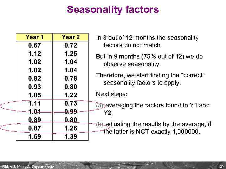Seasonality factors In 3 out of 12 months the seasonality factors do not match. But in 9 months (75% out of 12) we do observe seasonality. Therefore, we start finding the “correct” seasonality factors to apply. Next steps: (a) averaging the factors found in Y 1 and Y 2; (b) adjusting the results by the average, if the latter is NOT exactly 1, 000000. RM, v. 3/2011, A. Zaporozhetz 29

Seasonality factors RM, v. 3/2011, A. Zaporozhetz 30

4. Quantitative methods RM, v. 3/2011, A. Zaporozhetz 31

4. Quantitative methods: graphs RM, v. 3/2011, A. Zaporozhetz 32

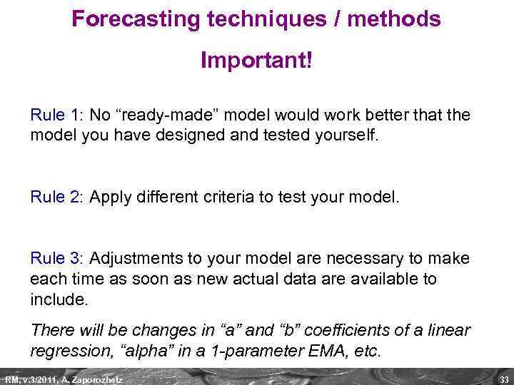Forecasting techniques / methods Important! Rule 1: No “ready-made” model would work better that the model you have designed and tested yourself. Rule 2: Apply different criteria to test your model. Rule 3: Adjustments to your model are necessary to make each time as soon as new actual data are available to include. There will be changes in “a” and “b” coefficients of a linear regression, “alpha” in a 1 -parameter EMA, etc. RM, v. 3/2011, A. Zaporozhetz 33

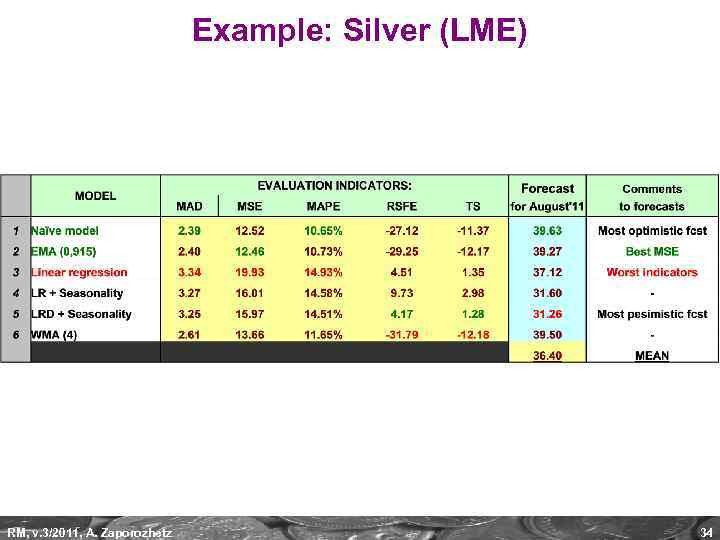Example: Silver (LME) RM, v. 3/2011, A. Zaporozhetz 34

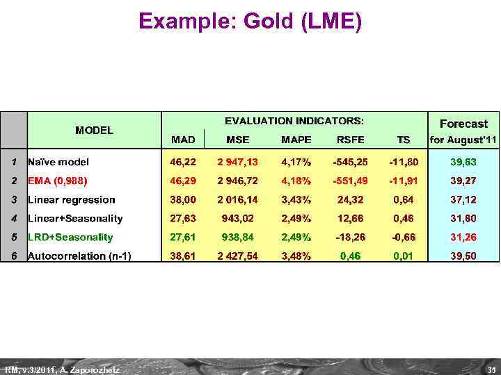Example: Gold (LME) RM, v. 3/2011, A. Zaporozhetz 35

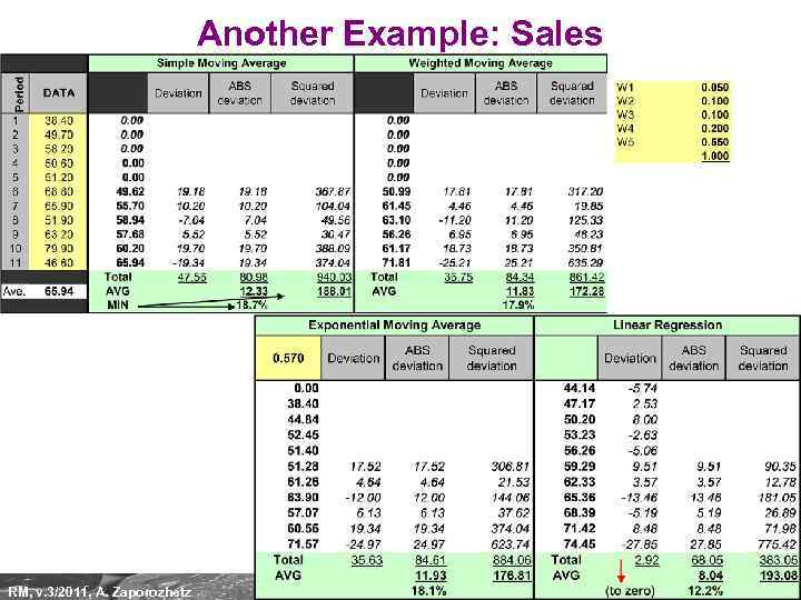Another Example: Sales RM, v. 3/2011, A. Zaporozhetz 36

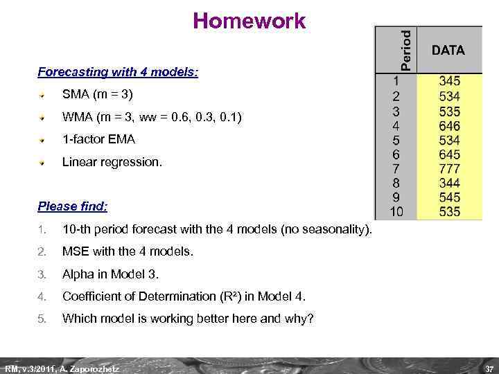Homework Forecasting with 4 models: SMA (m = 3) WMA (m = 3, ww = 0. 6, 0. 3, 0. 1) 1 -factor EMA Linear regression. Please find: 1. 10 -th period forecast with the 4 models (no seasonality). 2. MSE with the 4 models. 3. Alpha in Model 3. 4. Coefficient of Determination (R²) in Model 4. 5. Which model is working better here and why? RM, v. 3/2011, A. Zaporozhetz 37

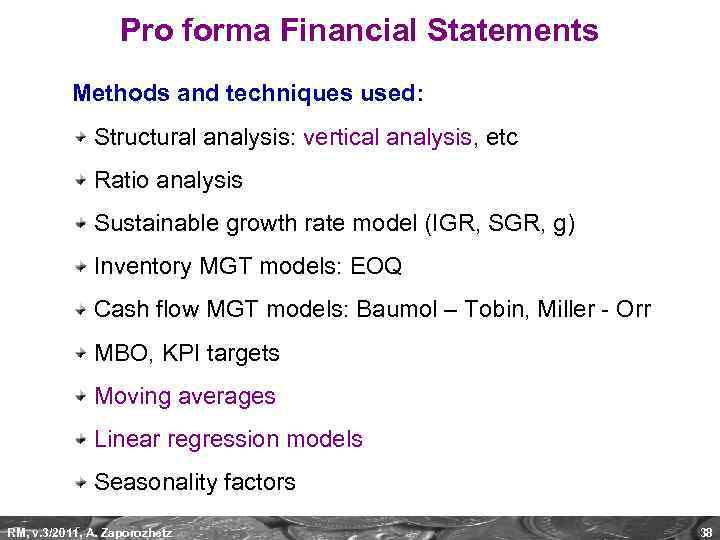Pro forma Financial Statements Methods and techniques used: Structural analysis: vertical analysis, etc Ratio analysis Sustainable growth rate model (IGR, SGR, g) Inventory MGT models: EOQ Cash flow MGT models: Baumol – Tobin, Miller - Orr MBO, KPI targets Moving averages Linear regression models Seasonality factors RM, v. 3/2011, A. Zaporozhetz 38