Class 2 Measuring Market Risk What does

Class 2 Measuring Market Risk

What does the company measure risk for? 2

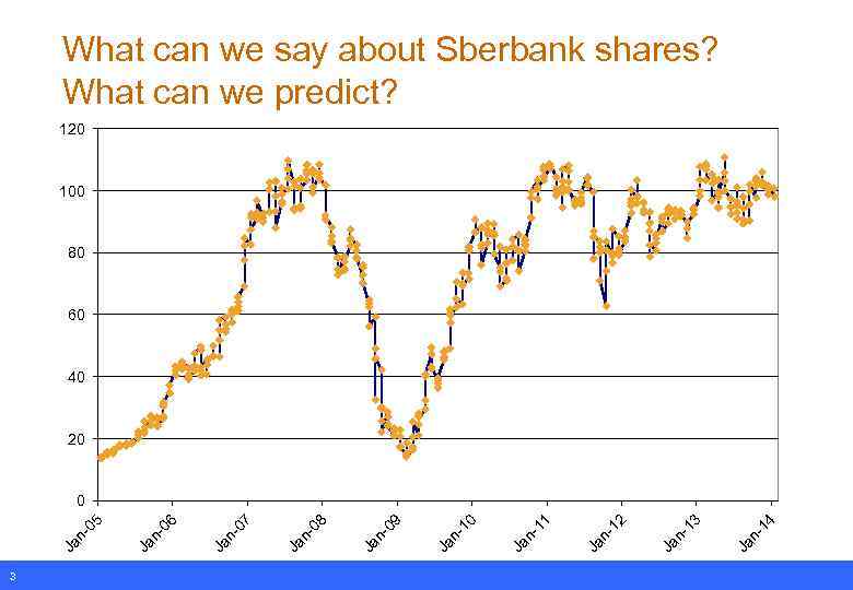What can we say about Sberbank shares? What can we predict? 120 100 80 60 40 20 3 Ja n 14 Ja n 13 Ja n 12 Ja n 11 Ja n 10 Ja n 09 Ja n 08 Ja n 07 Ja n 06 Ja n 05 0

What can we say about Sberbank shares? What can we predict? q Movements in asset prices are (almost) unpredictable – If someone could predict tomorrow’s price, (s)he would trade on this information and move today’s price to fair value – This is the basis for the Efficient Markets hypothesis q Prices move due to economic news arriving – Positive and negative news move the market up and down q Although we can’t predict future prices q …we can predict risk! 4

How to measure risk? q Size of the position – $XXX mln q Magnitude of price changes – Volatility: st. deviation / EWMA / GARCH q Sensitivity (exposure) to risk factors (indices) – Beta / duration / delta q Potential losses – Va. R / CVa. R (Expected Shortfall) 5

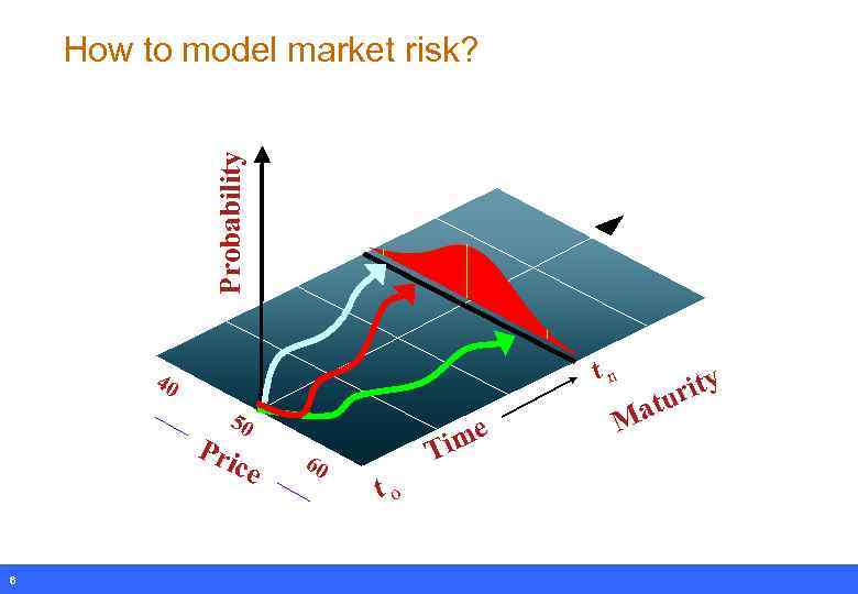Probability How to model market risk? tn 40 50 Pri 6 ce 60 me Ti to Ma rity tu

From prices to returns q Prices are convenient for graphical analysis, but. . – Non-stationary: properties of the stochastic process change over time – Must be corrected for dividends and stock splits q Thus, prices should be normalized to compare dynamics over time and across securities q Transforming prices into returns: Rt = (Pt+Dt-Pt-1)/Pt-1 – Return = percentage growth in the portfolio’s value, including capital gain and accumulated dividends/coupons 7

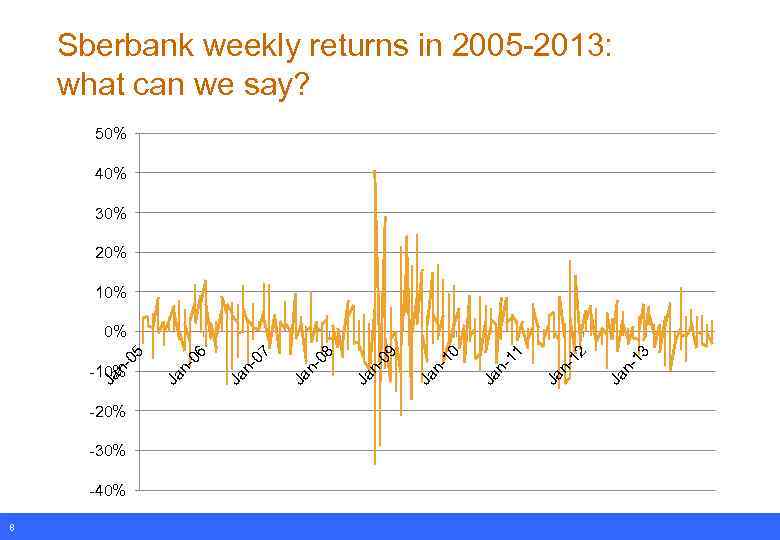Sberbank weekly returns in 2005 -2013: what can we say? 50% 40% 30% 20% 10% -20% -30% -40% 8 Ja n 1 3 2 n 1 Ja 11 Ja n- 0 n 1 Ja 9 n 0 Ja 8 n 0 Ja 7 n 0 Ja 6 n 0 Ja -10% Ja n 0 5 0%

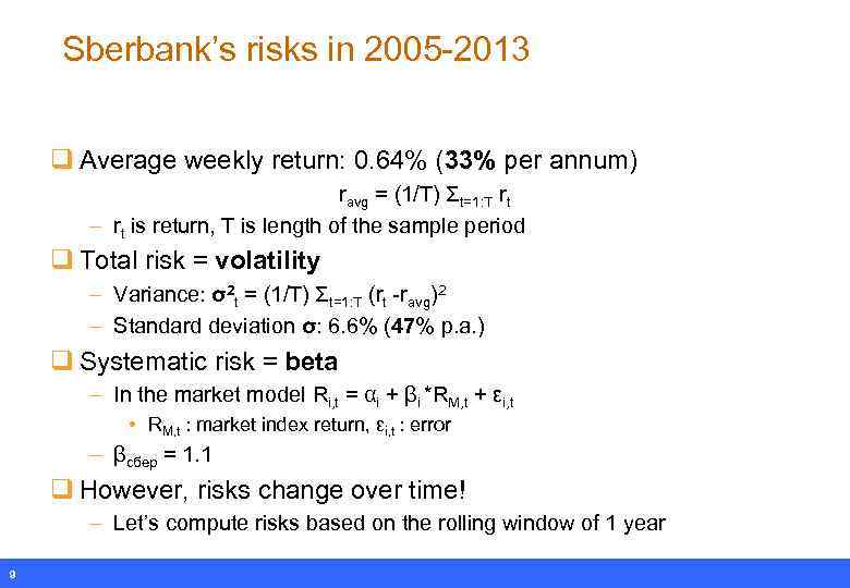Sberbank’s risks in 2005 -2013 q Average weekly return: 0. 64% (33% per annum) ravg = (1/T) Σt=1: T rt – rt is return, T is length of the sample period q Total risk = volatility – Variance: σ2 t = (1/T) Σt=1: T (rt -ravg)2 – Standard deviation σ: 6. 6% (47% p. a. ) q Systematic risk = beta – In the market model Ri, t = αi + βi *RM, t + εi, t • RM, t : market index return, εi, t : error – βсбер = 1. 1 q However, risks change over time! – Let’s compute risks based on the rolling window of 1 year 9

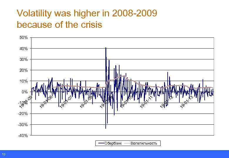Volatility was higher in 2008 -2009 because of the crisis 50% 40% 30% 20% 10% -20% -30% -40% Сбербанк 10 Волатильность -1 3 19 -0 1 -1 2 19 -0 1 -1 1 -0 1 19 01 -1 0 19 - 01 -0 9 19 - 01 -0 8 19 - -0 7 19 -0 1 01 -0 6 19 - -10% 19 - 01 -0 5 0%

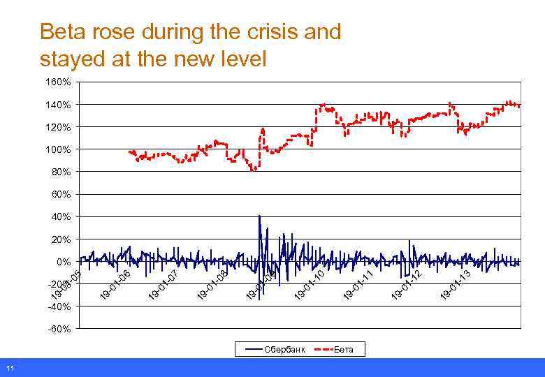Beta rose during the crisis and stayed at the new level 160% 140% 120% 100% 80% 60% 40% 20% -60% Сбербанк 11 Бета 01 -1 3 19 - 01 -1 2 19 - 01 -1 1 19 - -1 0 19 -0 1 -0 9 19 -0 1 -0 8 19 -0 1 -0 7 -0 1 19 -40% 01 -0 6 19 -0 1 -20% 19 - -0 5 0%

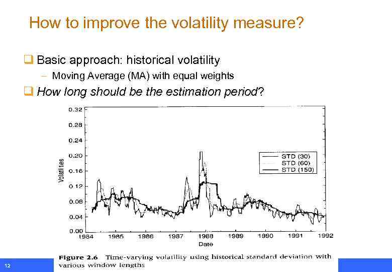How to improve the volatility measure? q Basic approach: historical volatility – Moving Average (MA) with equal weights q How long should be the estimation period? 12

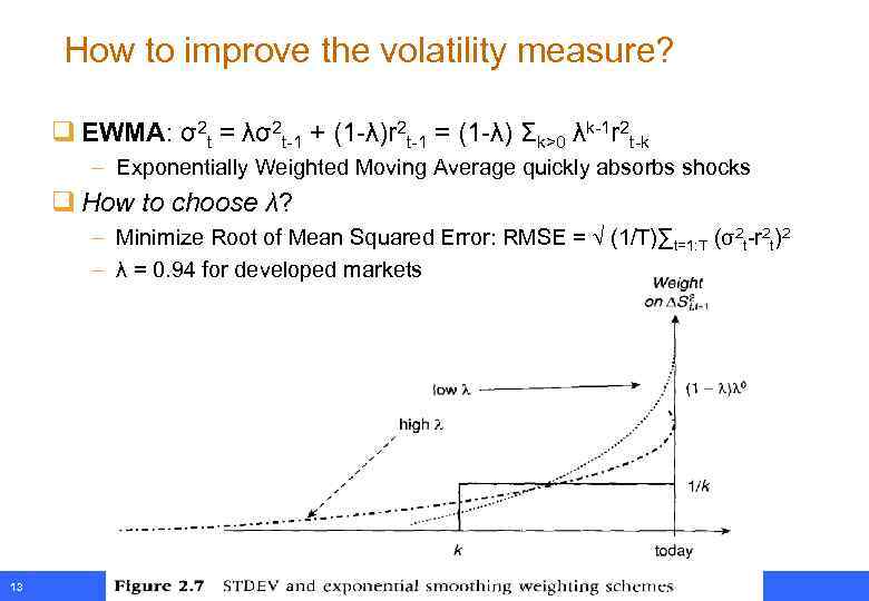How to improve the volatility measure? q EWMA: σ2 t = λσ2 t-1 + (1 -λ)r 2 t-1 = (1 -λ) Σk>0 λk-1 r 2 t-k – Exponentially Weighted Moving Average quickly absorbs shocks q How to choose λ? – Minimize Root of Mean Squared Error: RMSE = √ (1/T)∑t=1: T (σ2 t-r 2 t)2 – λ = 0. 94 for developed markets 13

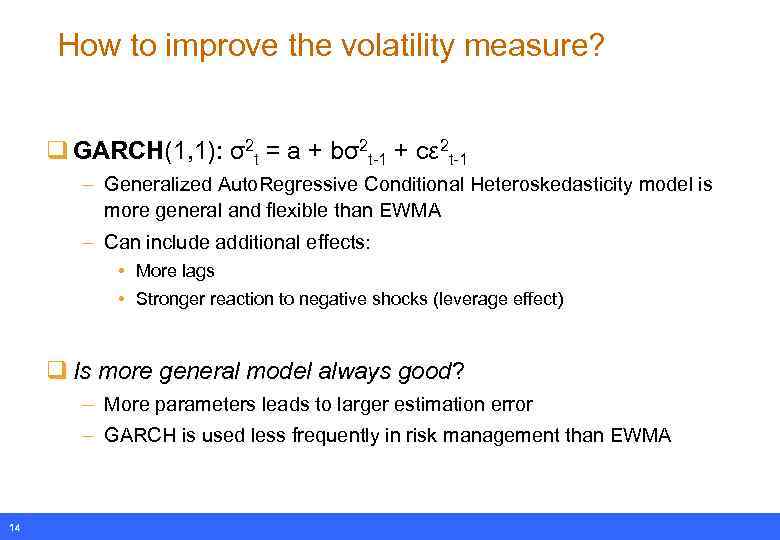How to improve the volatility measure? q GARCH(1, 1): σ2 t = a + bσ2 t-1 + cε 2 t-1 – Generalized Auto. Regressive Conditional Heteroskedasticity model is more general and flexible than EWMA – Can include additional effects: • More lags • Stronger reaction to negative shocks (leverage effect) q Is more general model always good? – More parameters leads to larger estimation error – GARCH is used less frequently in risk management than EWMA 14

How to improve the volatility measure? q Implied volatility: based on options’ market prices and (Black-Sholes) model 15 q Realized volatility: based on intraday data

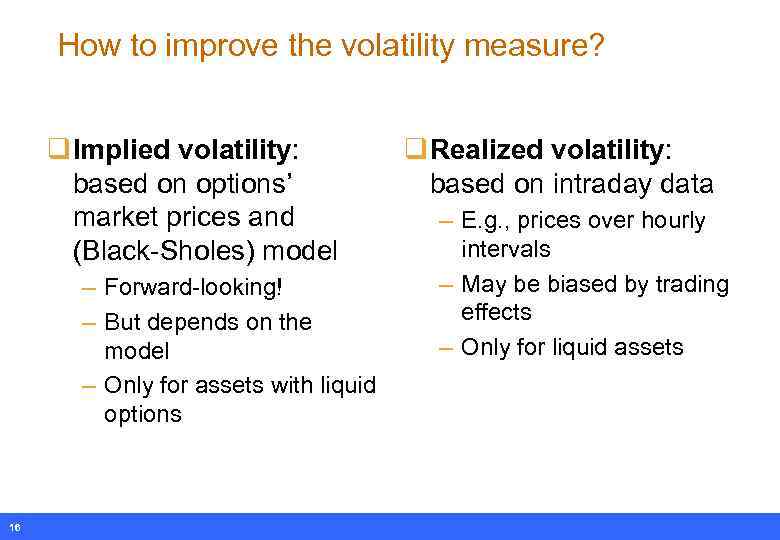How to improve the volatility measure? q Implied volatility: based on options’ market prices and (Black-Sholes) model – Forward-looking! – But depends on the model – Only for assets with liquid options 16 q Realized volatility: based on intraday data – E. g. , prices over hourly intervals – May be biased by trading effects – Only for liquid assets

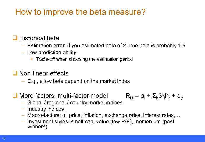How to improve the beta measure? q Historical beta – Estimation error: if you estimated beta of 2, true beta is probably 1. 5 – Low prediction ability • Trade-off when choosing the estimation period q Non-linear effects – E. g. , allow beta depend on the market index q More factors: multi-factor model – – 17 Ri, t = αi + Σkβki. Ikt + εi, t Global / regional / country market indices Industry indices Macro-factors: oil price, inflation, exchange rates, interest rates, … Investment styles: small-cap, value (low P/E), momentum (past winners)

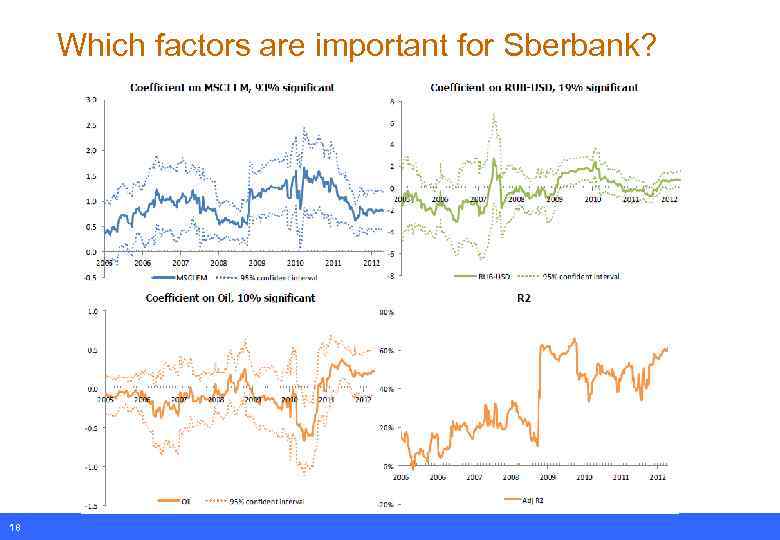Which factors are important for Sberbank? 18

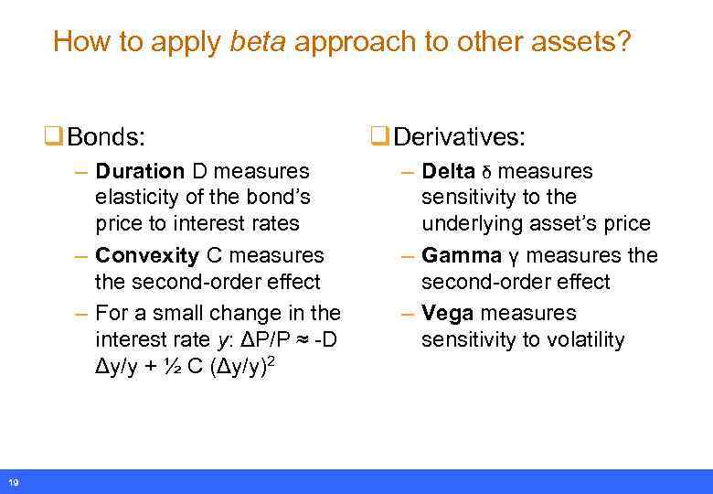How to apply beta approach to other assets? q Bonds: – Duration D measures elasticity of the bond’s price to interest rates – Convexity C measures the second-order effect – For a small change in the interest rate y: ΔP/P ≈ -D Δy/y + ½ C (Δy/y)2 19 q Derivatives: – Delta δ measures sensitivity to the underlying asset’s price – Gamma γ measures the second-order effect – Vega measures sensitivity to volatility

Why are volatility and beta not good enough? q Drawbacks of volatility – It measures speculative risk: both negative and positive deviations – It does not capture fat tails and asymmetry q Drawbacks of beta – Can’t capture non-linear effects (especially important for derivatives) – Ignores omitted risks q Even more important problems: – Communication: how to explain to your boss – Comparability of different types of risk 20

How to interpret Va. R? q Value-at-Risk measures potential losses – Maximum loss due to market fluctuations over a certain time period with a given probability (confidence level) Prob (Loss over 1 day < Va. R) = 95% – Risk. Metrics (original approach of investment banks) Prob (Loss over 10 days < Va. R) = 99% – Basel approach (banking regulators): larger confidence interval and holding period q What is a better confidence interval and holding period? – The higher the confidence level, the lower the precision – Holding period depends on time necessary to close or hedge the position 21

Method 1: Historical simulation q Nonparametric approach – Assuming that distribution of future returns is well approximated by the empirical distribution of returns over a certain period in the past q Applied directly to the asset: – Va. R = Percentile of historical returns – Easy way to get it: by sorting or plotting histogram q Applied to the portfolio: – Portfolio return = function of assets or risk factors • Must know portfolio weights, factor betas or price function (e. g. Black. Scholes) – Compute hypothetical historical returns of the current portfolio q Note: similar to bootstrap – Using past returns as possible scenarios

Critique: pros and cons q Easy and simple q Model-free – No need to assume normal distribution, forecast volatility q Correlations are embedded q Choice of the sample period – – Usually, at least 1 year Using short history, we may miss rare shocks q Slow reaction to changes in risks q Hard to extrapolate to a longer horizon

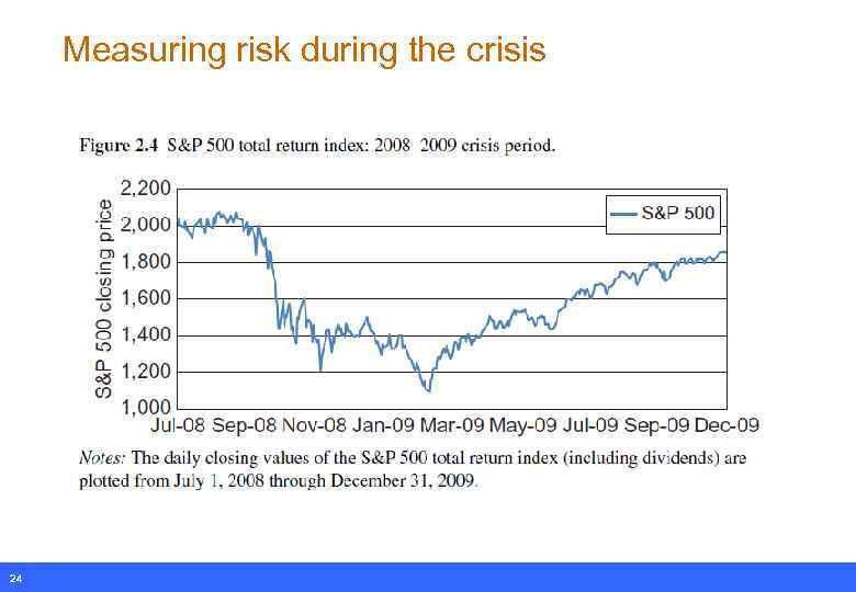Measuring risk during the crisis 24

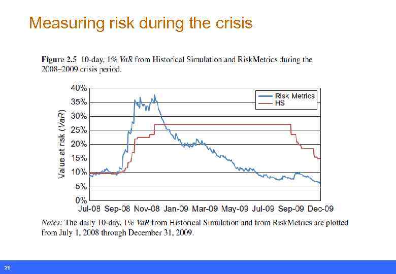Measuring risk during the crisis 25

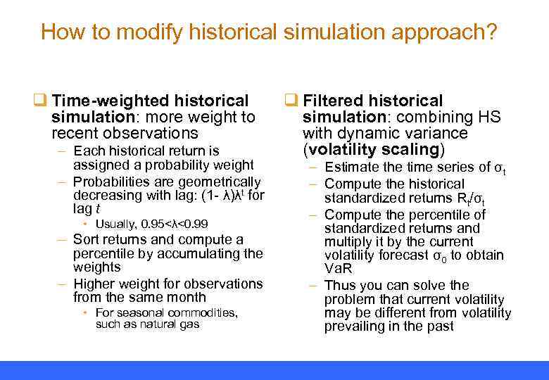How to modify historical simulation approach? q Time-weighted historical simulation: more weight to recent observations – Each historical return is assigned a probability weight – Probabilities are geometrically decreasing with lag: (1 - λ)λt for lag t • Usually, 0. 95<λ<0. 99 – Sort returns and compute a percentile by accumulating the weights – Higher weight for observations from the same month • For seasonal commodities, such as natural gas q Filtered historical simulation: combining HS with dynamic variance (volatility scaling) – Estimate the time series of σt – Compute the historical standardized returns Rt/σt – Compute the percentile of standardized returns and multiply it by the current volatility forecast σ0 to obtain Va. R – Thus you can solve the problem that current volatility may be different from volatility prevailing in the past

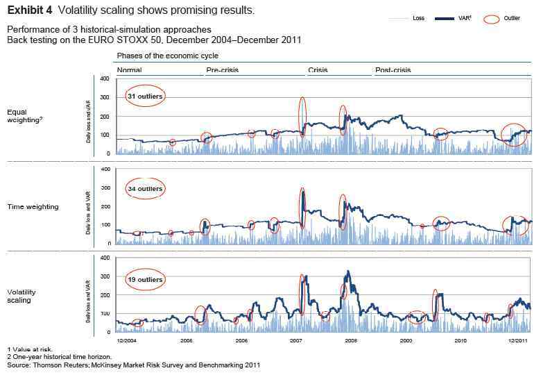27

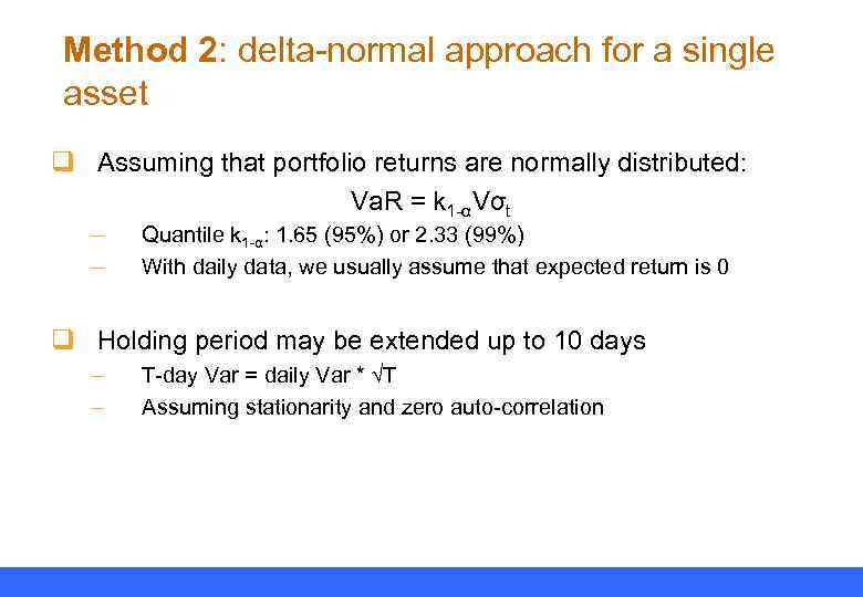Method 2: delta-normal approach for a single asset q Assuming that portfolio returns are normally distributed: Va. R = k 1 -αVσt – – Quantile k 1 -α: 1. 65 (95%) or 2. 33 (99%) With daily data, we usually assume that expected return is 0 q Holding period may be extended up to 10 days – – T-day Var = daily Var * √T Assuming stationarity and zero auto-correlation

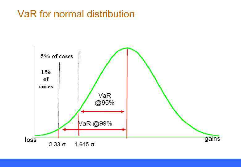Va. R for normal distribution

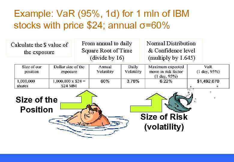Example: Va. R (95%, 1 d) for 1 mln of IBM stocks with price $24; annual σ=60% Calculate the $ value of the exposure Size of the Position From annual to daily Square Root of Time (divide by 16) Normal Distribution & Confidence level (multiply by 1. 645) Size of Risk (volatility)

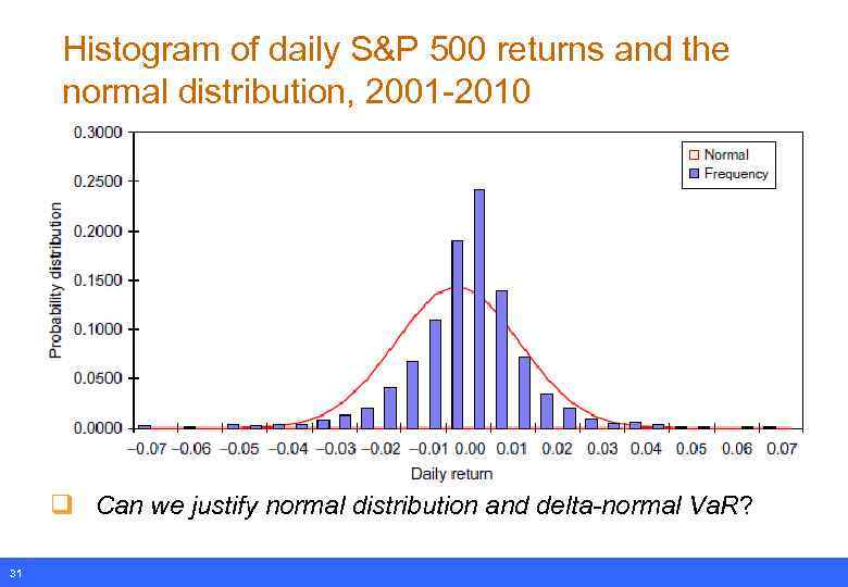Histogram of daily S&P 500 returns and the normal distribution, 2001 -2010 q Can we justify normal distribution and delta-normal Va. R? 31

Measuring risk during the crisis 32

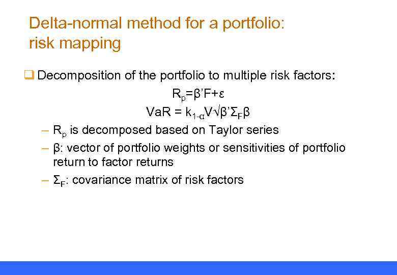Delta-normal method for a portfolio: risk mapping q Decomposition of the portfolio to multiple risk factors: Rp=β’F+ε Va. R = k 1 -αV√β’ΣFβ – Rp is decomposed based on Taylor series – β: vector of portfolio weights or sensitivities of portfolio return to factor returns – ΣF: covariance matrix of risk factors

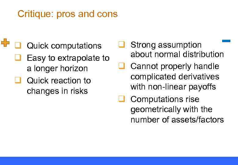Critique: pros and cons q Strong assumption q Quick computations about normal distribution q Easy to extrapolate to q Cannot properly handle a longer horizon complicated derivatives q Quick reaction to with non-linear payoffs changes in risks q Computations rise geometrically with the number of assets/factors

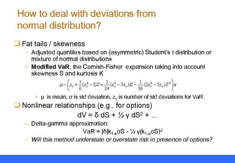How to deal with deviations from normal distribution? q Fat tails / skewness – Adjusted quantiles based on (asymmetric) Student’s t distribution or mixture of normal distributions – Modified Va. R: the Cornish-Fisher expansion taking into account skewness S and kurtosis K • μ is mean, σ is std deviation, zc is number of std deviations for Va. R q Nonlinear relationships (e. g. , for options) d. V = δ d. S + ½ γ d. S 2 +. . . – Delta-gamma approximation: Va. R = |δ|k 1 -ασS - ½ γ(k 1 -ασS)2 – Will this method understate or overstate risk in presence of options?

Method 3: Monte Carlo simulation q Model (multivariate) factor distributions – – Stocks: Geometric Brownian Motion / with jumps Interest rates: Vasicek / CIR / multifactor models q Generate scenarios and compute the realized P&L – Using factor innovations from the model q Plot and analyze the empirical distribution of P&L

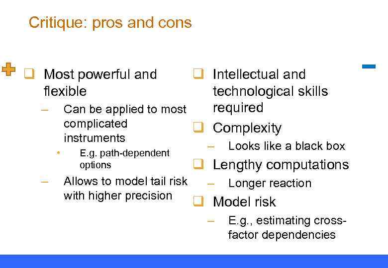Critique: pros and cons q Most powerful and flexible q Intellectual and technological skills required Can be applied to most complicated q Complexity – instruments • – E. g. path-dependent options Allows to model tail risk with higher precision – Looks like a black box q Lengthy computations – Longer reaction q Model risk – E. g. , estimating crossfactor dependencies

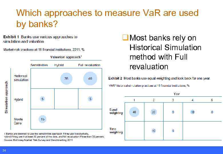Which approaches to measure Va. R are used by banks? q Most banks rely on Historical Simulation method with Full revaluation 38

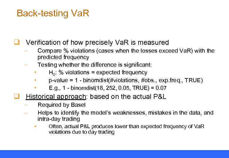Back-testing Va. R q Verification of how precisely Va. R is measured – – Compare % violations (cases when the losses exceed Va. R) with the predicted frequency Testing whether the difference is significant: • H 0: % violations = expected frequency • p-value = 1 - binomdist(#violations, #obs. , exp. freq. , TRUE) • E. g. , 1 - binomdist(18, 252, 0. 05, TRUE) = 0. 07 q Historical approach: based on the actual P&L – – Required by Basel Helps to identify the model’s weaknesses, mistakes in the data, and intra-day trading • Often, actual P&L produces lower than expected frequency of Va. R violations due to day trading

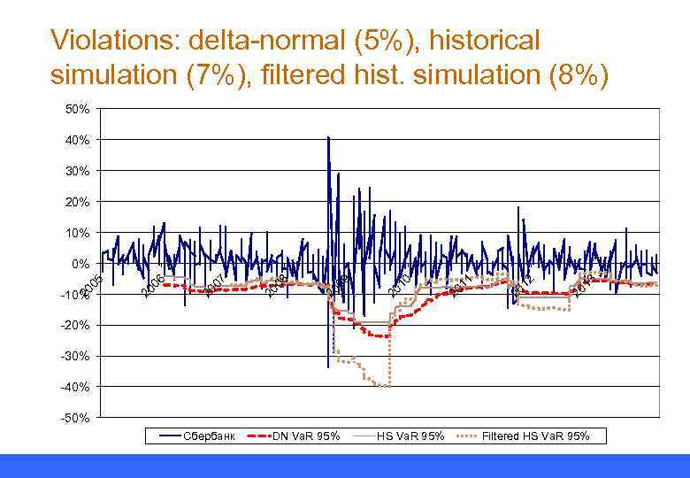Violations: delta-normal (5%), historical simulation (7%), filtered hist. simulation (8%) 50% 40% 30% 20% 13 20 12 20 11 20 10 20 09 20 08 20 07 06 20 20 -10% 20 05 0% -20% -30% -40% -50% Сбербанк DN Va. R 95% HS Va. R 95% Filtered HS Va. R 95%

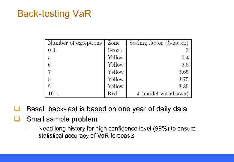Back-testing Va. R q Basel: back-test is based on one year of daily data q Small sample problem – Need long history for high confidence level (99%) to ensure statistical accuracy of Va. R forecasts

How else can we back-test different Va. R models (besides percentage of violations)? q Accuracy: the difference between VAR and actual daily P&L – An accurate model will be highly reactive, in the sense that it will rise and fall in a way that corresponds to daily fluctuations in the P&L. As a result, it will have high information content; management will be able to see changes in market conditions reflected quickly. Excess RWAs will be avoided, as VAR reduces rapidly when volatility declines. q Stability: the change in VAR from day to day – A stable model will not be prone to surprising leaps in VAR when risk positions change only slightly. – A stable model will avoid sudden drops in VAR when data points fall out of the time series and will not be overly reactive to small, short-term changes in market conditions. q Precision in predicting losses: mean violation 42