CIAR Summer School Tutorial Lecture 1 b Sigmoid

CIAR Summer School Tutorial Lecture 1 b Sigmoid Belief Nets Geoffrey Hinton

Discovering causal structure as a goal for unsupervised learning • It is better to associate responses with the hidden causes than with the raw data. • The hidden causes are useful for understanding the data. • It would be interesting if real neurons really did represent independent hidden causes.

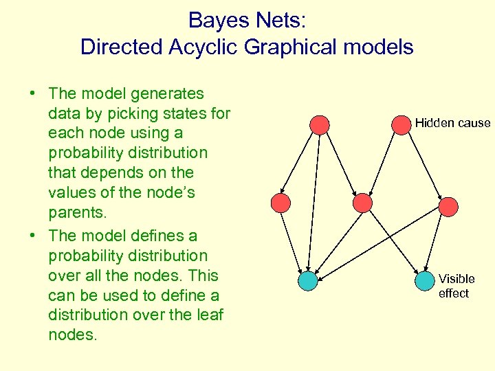
Bayes Nets: Directed Acyclic Graphical models • The model generates data by picking states for each node using a probability distribution that depends on the values of the node’s parents. • The model defines a probability distribution over all the nodes. This can be used to define a distribution over the leaf nodes. Hidden cause Visible effect

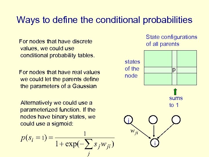
Ways to define the conditional probabilities State configurations of all parents For nodes that have discrete values, we could use conditional probability tables. For nodes that have real values we could let the parents define the parameters of a Gaussian Alternatively we could use a parameterized function. If the nodes have binary states, we could use a sigmoid: states of the node p sums to 1 j i

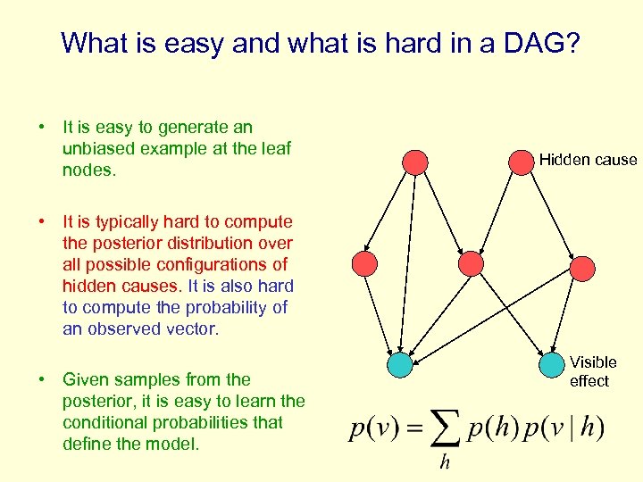
What is easy and what is hard in a DAG? • It is easy to generate an unbiased example at the leaf nodes. Hidden cause • It is typically hard to compute the posterior distribution over all possible configurations of hidden causes. It is also hard to compute the probability of an observed vector. • Given samples from the posterior, it is easy to learn the conditional probabilities that define the model. Visible effect

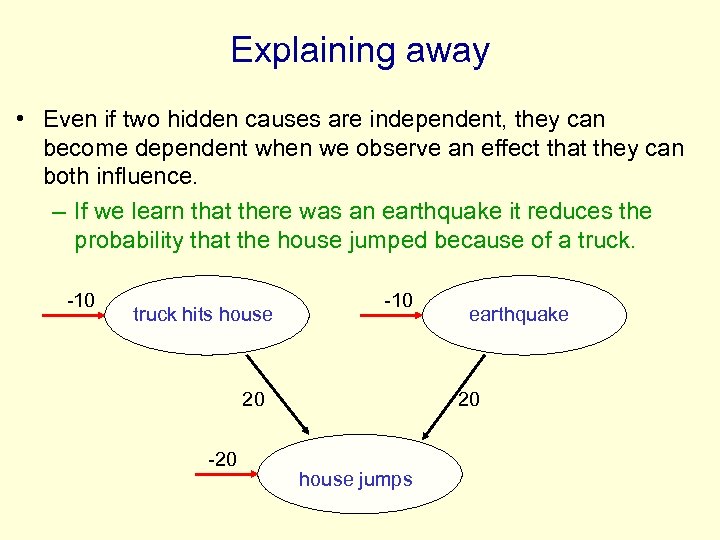
Explaining away • Even if two hidden causes are independent, they can become dependent when we observe an effect that they can both influence. – If we learn that there was an earthquake it reduces the probability that the house jumped because of a truck. -10 truck hits house -10 20 -20 earthquake 20 house jumps

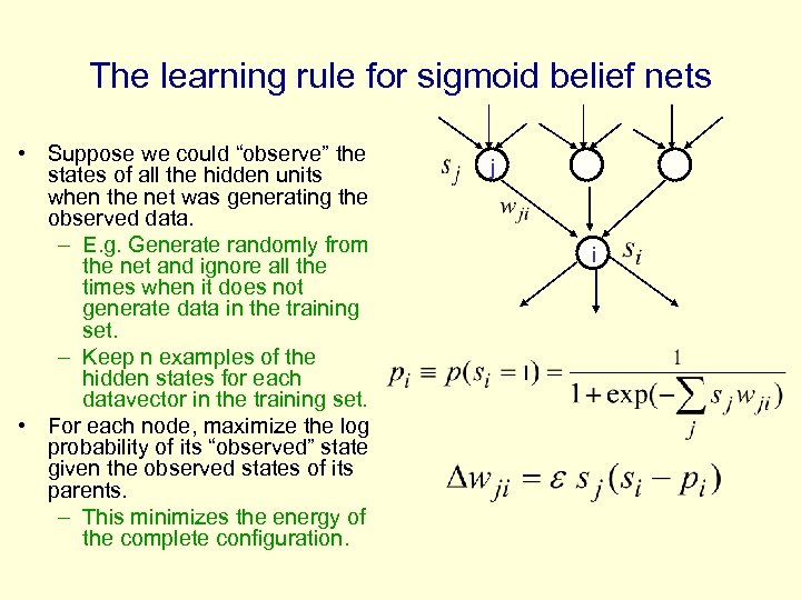
The learning rule for sigmoid belief nets • Suppose we could “observe” the states of all the hidden units when the net was generating the observed data. – E. g. Generate randomly from the net and ignore all the times when it does not generate data in the training set. – Keep n examples of the hidden states for each datavector in the training set. • For each node, maximize the log probability of its “observed” state given the observed states of its parents. – This minimizes the energy of the complete configuration. j i

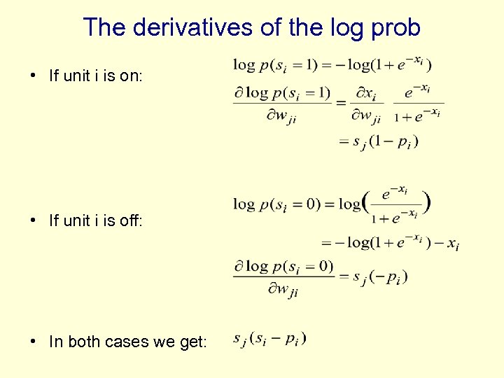
The derivatives of the log prob • If unit i is on: • If unit i is off: • In both cases we get:

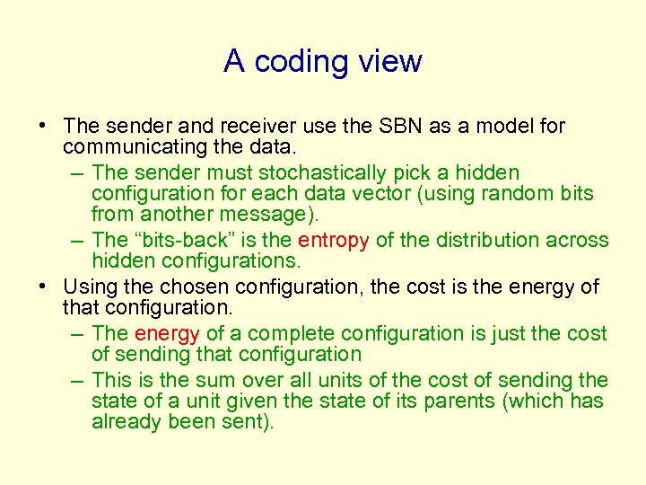
A coding view • The sender and receiver use the SBN as a model for communicating the data. – The sender must stochastically pick a hidden configuration for each data vector (using random bits from another message). – The “bits-back” is the entropy of the distribution across hidden configurations. • Using the chosen configuration, the cost is the energy of that configuration. – The energy of a complete configuration is just the cost of sending that configuration – This is the sum over all units of the cost of sending the state of a unit given the state of its parents (which has already been sent).

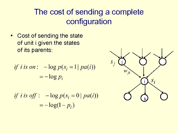
The cost of sending a complete configuration • Cost of sending the state of unit i given the states of its parents: j i k

Minimizing the coding cost • Pick hidden configurations using a Boltzmann distribution in their energies – This is exactly the posterior distribution over configurations given the datavector • Minimize the expected energy of the chosen configurations. – Change the parameters to minimize the energies of configurations weighted by their probability of being picked. • Don’t worry about the changes in the free energy caused by changes in the posterior distribution. – We chose the distribution to minimize free energy. – So small changes in the distribution have no effect on the free energy!

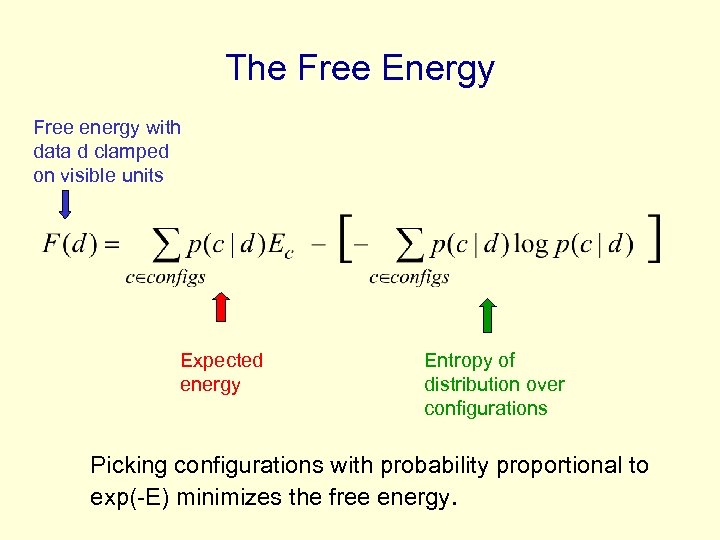
The Free Energy Free energy with data d clamped on visible units Expected energy Entropy of distribution over configurations Picking configurations with probability proportional to exp(-E) minimizes the free energy.

Sampling from the posterior distribution • In a densely connected sigmoid belief net with many hidden units it is intractable to compute the full posterior distribution over hidden configurations. – There are too many configurations to consider. • But we can learn OK if we just get samples from the posterior. – So how can we get samples efficiently? • Generating at random and rejecting cases that do not produce data in the training set is hopeless.

Gibbs sampling • First fix a datavector from the training set on the visible units. • Then keep visiting hidden units and updating their binary states using information from their parents and descendants. • If we do this in the right way, we will eventually get unbiased samples from the posterior distribution for that datavector. • This is relatively efficient because almost all hidden configurations will have negligible probability and will probably not be visited.

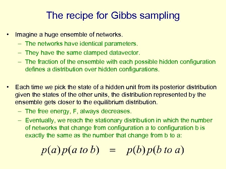
The recipe for Gibbs sampling • Imagine a huge ensemble of networks. – The networks have identical parameters. – They have the same clamped datavector. – The fraction of the ensemble with each possible hidden configuration defines a distribution over hidden configurations. • Each time we pick the state of a hidden unit from its posterior distribution given the states of the other units, the distribution represented by the ensemble gets closer to the equilibrium distribution. – The free energy, F, always decreases. – Eventually, we reach the stationary distribution in which the number of networks that change from configuration a to configuration b is exactly the same as the number that change from b to a:

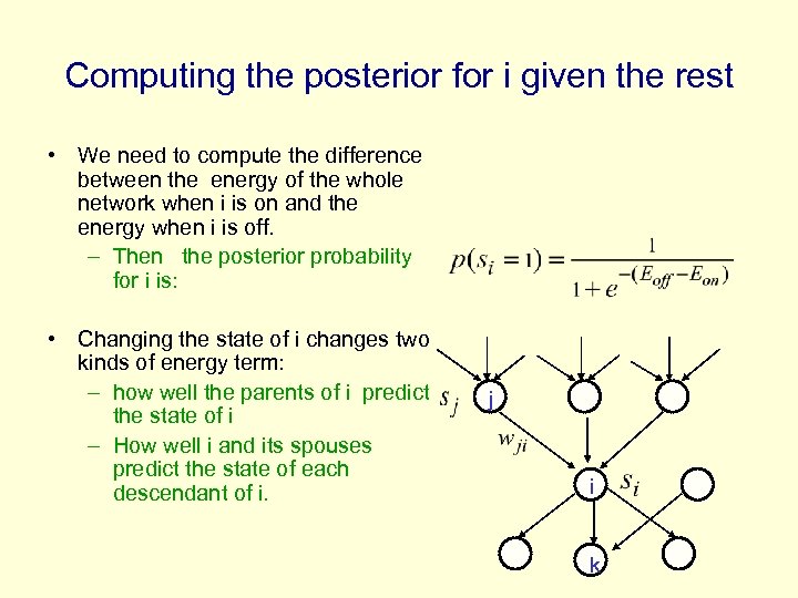
Computing the posterior for i given the rest • We need to compute the difference between the energy of the whole network when i is on and the energy when i is off. – Then the posterior probability for i is: • Changing the state of i changes two kinds of energy term: – how well the parents of i predict the state of i – How well i and its spouses predict the state of each descendant of i. j i k

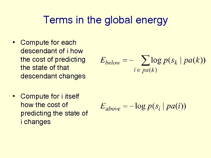
Terms in the global energy • Compute for each descendant of i how the cost of predicting the state of that descendant changes • Compute for i itself how the cost of predicting the state of i changes

Approximate inference • What if we use an approximation to the posterior distribution over hidden configurations? – e. g. assume the posterior factorizes into a product of distributions for each separate hidden cause. • If we use the approximation for learning, there is no guarantee that learning will increase the probability that the model would generate the observed data. • But maybe we can find a different and sensible objective function that is guaranteed to improve at each update.

The Free Energy Free energy with data d clamped on visible units Expected energy Entropy of distribution over configurations Picking configurations with probability proportional to exp(-E) minimizes the free energy.

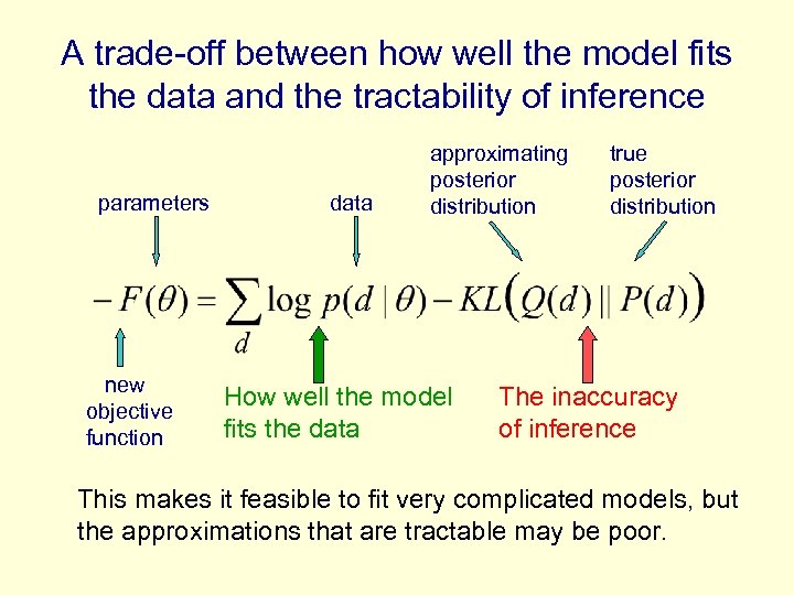
A trade-off between how well the model fits the data and the tractability of inference parameters new objective function data approximating posterior distribution How well the model fits the data true posterior distribution The inaccuracy of inference This makes it feasible to fit very complicated models, but the approximations that are tractable may be poor.

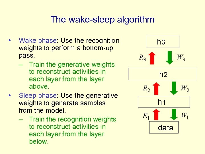
The wake-sleep algorithm • • Wake phase: Use the recognition weights to perform a bottom-up pass. – Train the generative weights to reconstruct activities in each layer from the layer above. Sleep phase: Use the generative weights to generate samples from the model. – Train the recognition weights to reconstruct activities in each layer from the layer below. h 3 h 2 h 1 data

What the wake phase achieves • The bottom-up recognition weights are used to compute a sample from the distribution Q over hidden configurations. Q approximates the true posterior, P. – In each layer Q assumes the states are independent given the states in the layer below. It ignores explaining away. • The changes to the generative weights are designed to reduce the average cost (i. e. energy) of generating the data when the hidden configurations are sampled from the approximate posterior. – The updates to the generative weights follow the gradient of the variational bound with respect to the parameters of the model.

The flaws in the wake-sleep algorithm • The recognition weights are trained to invert the generative model in parts of the space where there is no data. – This is wasteful. • The recognition weights follow the gradient of the wrong divergence. They minimize KL(P||Q) but the variational bound requires minimization of KL(Q||P). – This leads to incorrect mode-averaging.

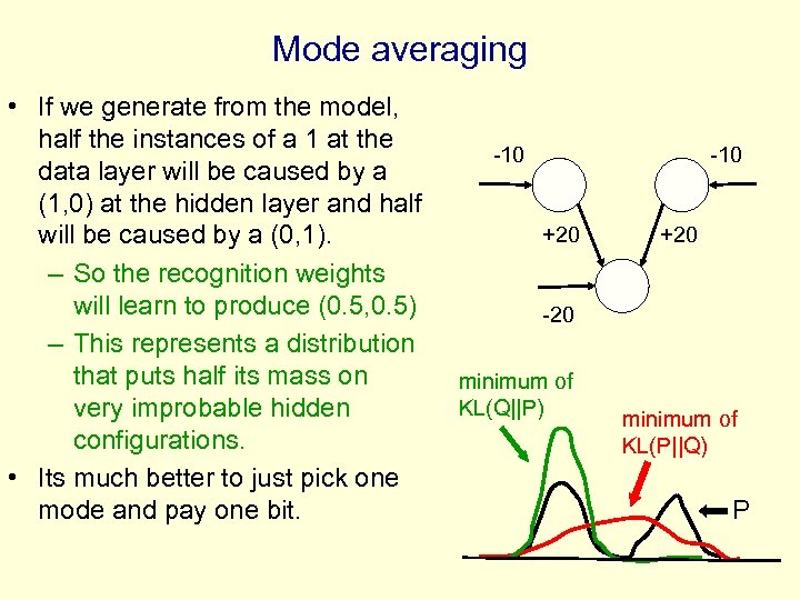
Mode averaging • If we generate from the model, half the instances of a 1 at the data layer will be caused by a (1, 0) at the hidden layer and half will be caused by a (0, 1). – So the recognition weights will learn to produce (0. 5, 0. 5) – This represents a distribution that puts half its mass on very improbable hidden configurations. • Its much better to just pick one mode and pay one bit. -10 +20 -20 minimum of KL(Q||P) minimum of KL(P||Q) P

Summary • By using the variational bound, we can learn sigmoid belief nets quickly. • If we add bottom-up recognition connections to a generative sigmoid belief net, we get a nice neural network model that requires a wake phase and a sleep phase. – The activation rules and the learning rules are very simple in both phases. This makes neuroscientists happy. • But there are problems: – The learning of the recognition weights in the sleep phase is not quite following the gradient of the variational bound. – Even if we could follow the right gradient, the variational approximation might be so crude that it severely limits what we can learn. • Variational learning works because the learning tries to find regions of the parameter space in which the variational bound is fairly tight, even if this means getting a model that gives lower log probability to the data.