Characterization of Planets Mass and Radius Transits Results

Characterization of Planets: Mass and Radius (Transits Results Part I) I. III. IV. Results from individual transit search programs Interesting cases Global Properties Spectroscopic Transits

The first time I gave this lecture (2003) there was one transiting extrasolar planet There are now 59 transiting extrasolar planets First ones were detected by doing follow-up photometry of radial velocity planets. Now transit searches are discovering exoplanets

Radial Velocity Curve for HD 209458 Period = 3. 5 days Msini = 0. 63 MJup

Charbonneau et al. (2000): The observations that started it all: • Mass = 0, 63 MJupiter • Radius = 1, 35 RJupiter • Density = 0, 38 g cm– 3

Transit detection was made with the 10 cm STARE Telescope

A light curve taken by amateur astronomers…

. . and by the Profis ( Hubble Space Telescope).

HD 209458 b has a radius larger than expected. Burrows et al. 2000 Evolution of the radius of HD 209458 b and t Boob HD 209458 b Models I, C, and D are for isolated planets Models A and B are for irradiated planets. One hypothesis for the large radius is that the stellar radiation hinders the contraction of the planet (it is hotter than it should be) so that it takes longer to contract. Another is tidal heating of the core of the planet if you have nonzero eccentricity

Successful Transit Search Programs • OGLE: Optical Gravitational Lens Experiment (http: //www. astrouw. edu. pl/~ogle/) • 1. 3 m telescope looking into the galactic bulge • Mosaic of 8 CCDs: 35‘ x 35‘ field • Typical magnitude: V = 15 -19 • Designed for Gravitational Microlensing • First planet discovered with the transit method • 8 Transiting planets discovered so far

The first planet found with the transit method

Konacki et al. Until this discovery radial velocity surveys only found planets with periods no shorter than 3 days. About ½ of the OGLE planets have periods less than 2 days.

M = 1. 03 MJup R = 1. 36 Rjup Period = 3. 7 days

Vsini = 40 km/s K = 510 170 m/s One reason I do not like OGLE transiting planets. These produce low quality transits, they are faint, and they take up a large amount of 8 m telescope time. i= 79. 8 0. 3 a= 0. 0308 Mass = 4. 5 MJ Radius = 1. 6 RJ Spectral Type = F 3 V

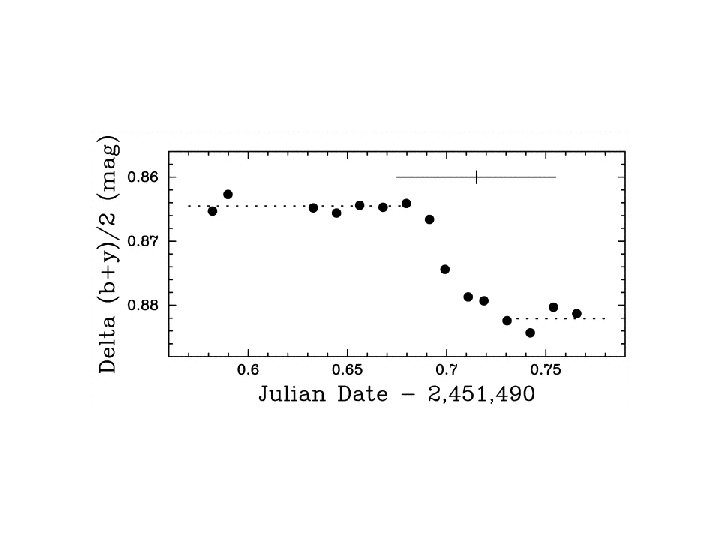
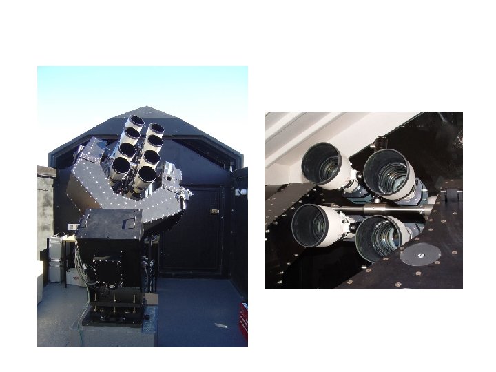
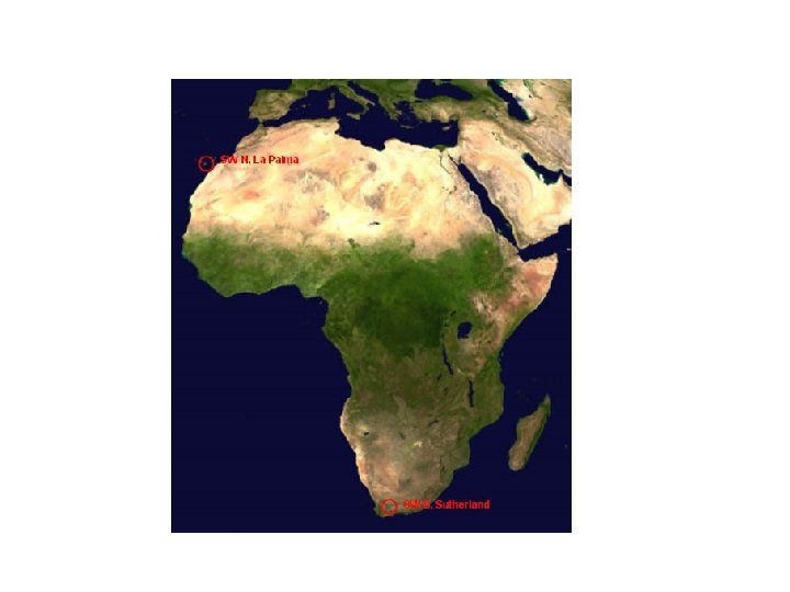
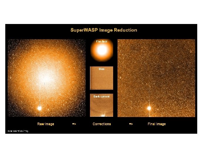
Successful Transit Search Programs WASP: Wide Angle Search for Planets (http: //www. superwasp. org). Also known as Super. WASP • Array of 8 Wide Field Cameras • Field of View: 7. 8 o x 7. 8 o • 13. 7 arcseconds/pixel • Typical magnitude: V = 9 -13 • 15 transiting planets discovered so far

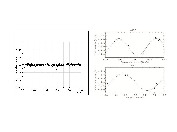
Coordinates RA 00: 20: 40. 07 Dec +31: 59: 23. 7 Constellation Pegasus Apparent Visual Magnitude 11. 79 Distance from Earth 1234 Light Years WASP-1 Spectral Type F 7 V WASP-1 Photospheric Temperature 6200 K WASP-1 b Radius 1. 39 Jupiter Radii WASP-1 b Mass 0. 85 Jupiter Masses Orbital Distance 0. 0378 AU Orbital Period 2. 52 Days Atmospheric Temperature 1800 K Mid-point of Transit 2453151. 4860 HJD

WASP 12: Hottest (at the time) Transiting Planet High quality light curve for accurate parameters Discovery data Orbital Period: 1. 09 d Transit duration: 2. 6 hrs Planet Mass: 1. 41 MJupiter Planet Radius: 1. 79 RJupiter Doppler confirmation Planet Temperature: 2516 K Spectral Type of Host Star: F 7 V

Comparison of WASP 12 to an M 8 Main Sequence Star Planet Mass: 1. 41 MJupiter Mass: 60 MJupiter Planet Radius: 1. 79 RJupiter Radius: 1 RJupiter Planet Temperature: 2516 K Teff: ~ 2800 K WASP 12 has a smaller mass, larger radius, and comparable effective temperature than an M 8 dwarf. Its atmosphere should look like an M 9 dwarf or L 0 brown dwarf

Mass – Radius Relationship Stars Planets

Successful Transit Search Programs • Tr. ES: Trans-atlantic Exoplanet Survey (STARE is a member of the network http: //www. hao. ucar. edu/public/research/stare/) • Three 10 cm telescopes located at Lowell Observtory, Mount Palomar and the Canary Islands • 6. 9 square degrees • 4 Planets discovered

Tr. Es 1 b

Tr. Es 2 b P = 2. 47 d M = 1. 28 MJupiter R = 1. 24 RJupiter i = 83. 9 deg

Successful Transit Search Programs • HATNet: Hungarian-made Automated Telescope (http: //www. cfa. harvard. edu/~gbakos/HAT/ • Six 11 cm telescopes located at two sites: Arizona and Hawaii • 8 x 8 square degrees • 12 Planets discovered

HAT-P-1 b Follow-up with larger telescope

HAT-P-1 b has an anomolously large radius for its mass

HAT-P-12 b Star = K 4 V Planet Period = 3. 2 days Planet Radius = 0. 96 RJup Planet Mass = 0. 21 MJup (~MSat) r = 0. 3 gm cm– 3

Special Transits: GJ 436 Host Star: Mass = 0. 4 M ( סּ M 2. 5 V) Butler et al. 2004

Special Transits: GJ 436 Butler et al. 2004 „Photometric transits of the planet across the star are ruled out for gas giant compositions and are also unlikely for solid compositions“

The First Transiting Hot Neptune Gillon et al. 2007

Special Transits: GJ 436 Star Stellar mass [ M ] סּ 0. 44 ( ± 0. 04) Planet Period [days] 2. 64385 ± 0. 00009 Eccentricity 0. 16 ± 0. 02 Orbital inclination 86. 5 0. 2 Planet mass [ ME ] 22. 6 ± 1. 9 Planet radius [ RE ] 3. 95 +0. 41 -0. 28 Mean density = 1. 95 gm cm– 3, in between Neptune (1. 58) and Uranus (2. 3)

Special Transits: HD 17156 M = 3. 11 MJup Probability of a transit ~ 3%

Barbieri et al. 2007 R = 0. 96 RJup Mean density = 4. 88 gm/cm 3 Mean for M 2 star ≈ 4. 3 gm/cm 3

Special Transits: HD 149026 Sato et al. 2005 Period = 2. 87 d Rp = 0. 7 RJup Mp = 0. 36 MJup Mean density = 2. 8 gm/cm 3

So what do all of these transiting planets tell us?

The density is the first indication of the internal structure of the exoplanet Solar System Object r (gm cm– 3) Mercury 5. 43 Venus 5. 24 Earth 5. 52 Mars 3. 94 Jupiter 1. 33 Saturn 0. 70 Uranus 1. 30 Neptune 1. 76 Pluto 2 Moon 3. 34 Carbonaceous Meteorites 2– 3. 5 Iron Meteorites 7– 8 Comets 0. 06 -0. 6

Mass Radius Relationship HD 209458 b and HAT-P-1 b have anomalously large radii that still cannot be explained by planetary structure and evolution models

HAT-12 b Co. Ro. T-3

10 -13 Mearth core ~70 Mearth core mass is difficult to form with gravitational instability. HD 149026 b provides strong support for the core accretion theory Rp = 0. 7 RJup Mp = 0. 36 MJup Mean density = 2. 8 gm/cm 3

GJ 436 b (transiting Neptune) has a density comparable to Uranus and Neptune and thus we expect similar structure

Take your favorite composition and calculate the mass-radius relationship

5 U e 5 – 2 4 % 75 % H H GJ 436 N 3 s Ice R/RE s ate ilic S 2 Fe 1 1 10 M/ME 100 The type of planet you have (rock versus iron, etc) is driven largely by the radius determination. E. g. : a silicate planet can have a mass that varies by more than 20%. A 20% error in the radius determines whether the planet is a rock or a piece of iron. This is because density ~ M, but R– 3

To get a better estimate of the composition of an exoplanet, you need to know the radius of the planet to within 5% or better • You need accurate transit depths → you should probably do this from space, or lots of measurements from the ground • You only determine Rplanet/Rstar. This means you need to know the radius of the star to within a few percent. For accurate stellar radii you must use - Interferometry - Asteroseismology

HAT-P-12 b The best fitting model for HAT-P-12 b has a core mass ≤ 10 Mearth and is still dominated by H/He (i. e. like Saturn and Jupiter and not like Uranus and Neptune. It is the lowest mass H/He dominated gas giant planet.

Global Properties

Planet Radius Most transiting planets tend to be inflated

Mass-Radius Relationship Radius is roughly independent of mass, until you get to small planets (rocks)

Mass of the Host Star Transiting Planets: 45% Stars have mass greater that 1 Msun However, probability of a transit is ~ Rstar/a, so this might be a selection effect. All Planets (mostly from Doppler surveys). 37% stars have mass greater than 1 Msun

Planet Mass Distribution It is rare to find close-in planets that have high mass, but they do exist. Some with masses up to 20 MJup (Co. Ro. T-3)

The Planet-Metallicity Connection Astronomer‘s Metals More Metals ! Even more Metals !!

Bracket Fe/H notation : [Fe/H] This is the ratio of metal abundance to the solar value. Often it is for Iron lines, but sometimes other heavy elements are included. Sometimes [M/H] is used for metals: [Fe/H] is calculated by taking the iron abundance, divide it by the abundance of iron in the sun, and then taking the logarithm base 10. [Fe/H] = 0 → solar abundance [Fe/H] = +0. 5 → 3. 16 × solar [Fe/H] = – 1. 0 → 0. 1 × solar Most metal rich stars have [Fe/H] = +0. 5, most metal poor have [Fe/H] ≈ – 3

The Planet-Metallicity Connection? These are stars with metallicity [Fe/H] ~ +0. 3 – +0. 5 Valenti & Fischer There is believed to be a connection between metallicity and planet formation. Stars with higher metalicity tend to have a higher frequency of planets. This has been used as evidence in support of the core accretion theory

Comparison of Metalicity Transiting Planets All Planets (mostly from Doppler surveys)

% Metallicity of Giant Stars also show no metallicity effect [Fe/H] Most planets around giant stars and transiting planets are for 1. 2 -1. 4 MSun host stars. And there seems to be no metallicity effect. Red line: Main sequence (1 solar mass) Blue: Giants (~1. 4 solar mass)

More problems with Planet – Metallicity Connection Endl et al. 2007: HD 155358 two planets and. . Hyades stars have [Fe/H] = 0. 2 and according to V&F relationship 10% of the stars should have giant planets, but none have been found in a sample of 100 stars …[Fe/H] = – 0. 68. This certainly muddles the metallicity-planet connection

• Early indications are that the host stars of transiting planets have different properties than non-transiting planets. • Most likely explanation: Transit searches are not as biased as radial velocity searches. One looks for transits around all stars in a field, these are not preselected. The only bias comes with which ones are followed up with Doppler measurements • Caveat: Transit searches are biased against smaller stars. i. e. the larger the star the higher probability that it transits

Spectroscopic Transits: The Rossiter-Mc. Claughlin Effect 2 1 +v 1 0 4 3 4 2 –v 3 The R-M effect occurs in eclipsing systems when the companion crosses in front of the star. This creates a distortion in the normal radial velocity of the star. This occurs at point 2 in the orbit.

The Rossiter-Mc. Laughlin Effect in an Eclipsing Binary From Holger Lehmann

The effect was discovered in 1924 independently by Rossiter and Mc. Claughlin Curves show Radial Velocity after removing the binary orbital motion

The Rossiter-Mc. Laughlin Effect or „Rotation Effect“ For rapidly rotating stars you can „see“ the planet in the spectral line

For stars whose spectral line profiles are dominated by rotational broadening there is a one to one mapping between location on the star and location in the line profile: V = –Vrot V = +Vrot V=0

A „Doppler Image“ of a Planet For slowly rotationg stars you do not see the distortion, but you measure a radial velocity displacement due to the distortion.

The Rossiter-Mc. Claughlin Effect –v +v 0 As the companion crosses the star the observed radial velocity goes from + to – (as the planet moves towards you the star is moving away). The companion covers part of the star that is rotating towards you. You see more possitive velocities from the receeding portion of the star) you thus see a displacement to + RV. +v –v When the companion covers the receeding portion of the star, you see more negatve velocities of the star rotating towards you. You thus see a displacement to negative RV.

Amplitude of the R-M effect: ARV = 52. 8 m s– 1 ( Vs 5 km s– 1 )( r 2 ) RJup ( R R סּ – 2 ) ARV is amplitude after removal of orbital mostion Vs is rotational velocity of star in km s– 1 r is radius of planet in Jupiter radii R is stellar radius in solar radii Note: 1. The Magnitude of the R-M effect depends on the radius of the planet and not its mass. 2. The R-M effect is proportional to the rotational velocity of the star. If the star has little rotation, it will not show a R-M effect.

The Rossiter-Mc. Claughlin Effect What can the RM effect tell you? 1. The inclination of „impact parameter“ –v –v +v +v Shorter duration and smaller amplitude

The Rossiter-Mc. Claughlin Effect What can the RM effect tell you? 2. Is the companion orbit in the same direction as the rotation of the star? –v +v +v –v

l What can the RM effect tell you? 3. Are the spin axes aligned? Orbital plane

Tr. ES-1

Results from the Rossiter-Mc. Claughlin Effect So far most transiting planets for which an RM effect has been measured has shown prograde orbits What about misalignment of the spin axis?

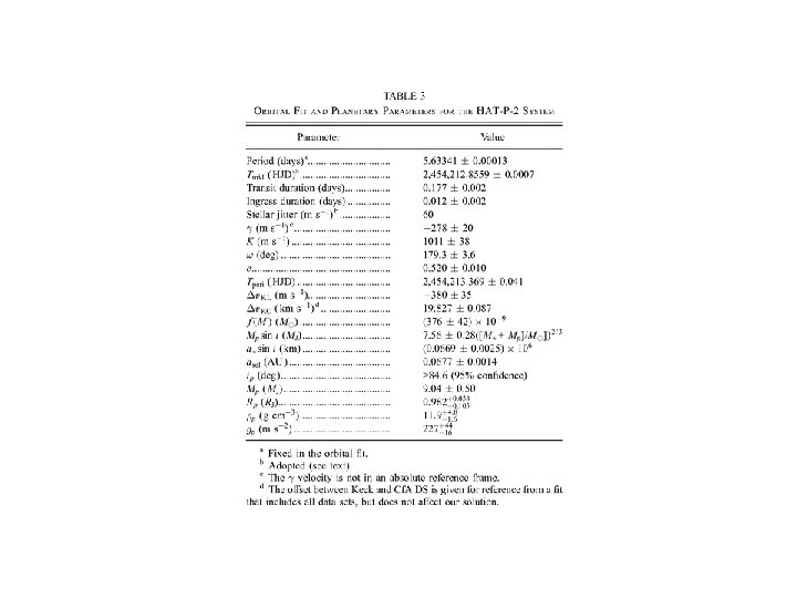
HD 147506 Best candidate for misalignment is HD 147506 because of the high eccentricity

On the Origin of the High Eccentricities Two possible explanations for the high eccentricities seen in exoplanet orbits: • Scattering by multiple giant planets • Kozai mechanism

Planet-Planet Interactions Initially you have two giant planets in circular orbits These interact gravitationally. One is ejected and the remaining planet is in an eccentric orbit

This mechanism has been invoked to explain the „massive eccentrics“ Recall that there are no massive planets in circular orbits

Kozai Mechanism Two stars are in long period orbits around each other. A planet is in a shorter period orbit around one star. If the orbit of the planet is inclined, the outer planet can „pump up“ the eccentricity of the planet. Planets can go from circular to eccentric orbits. This was first investigated by Kozai who showed that satellites in orbit around the Earth can have their orbital eccentricity changed by the gravitational influence of the Moon

Kozai Mechanism The Kozai mechanism has been used to explain the high orbital eccentricity of 16 Cyg B, a planet in a binary system

If either mechanism is at work, then we should expect that planets in eccentric orbits not have the spin axis aligned with the stellar rotation. This can be checked with transiting planets in eccentric orbits Winn et al. 2007: HD 147506 b (alias HAT-P-2 b) Spin axes are aligned within 14 degrees (error of measurement). No support for Kozai mechanism or scattering

What about HD 17156? Narita et al. (2007) reported a large (62 ± 25 degree) misalignment between planet orbit and star spin axes!

Cochran et al. 2008: l = 9. 3 ± 9. 3 degrees → No misalignment!

Fabricky & Winn, 2009, Ap. J, 696, 1230

XO-3 -b

Hebrard et al. 2008 l = 70 degrees

Winn et al. (2009) recent R-M measurements for X 0 -3 l = 37 degrees

Possible inclination changes in Tr. Es-2 Evidence that transit duration has decreased by 3. 2 minutes. This might be caused by inclination changes induced by a third body The biggest effect should be for grazing transits

Transit Timing Variations (TTVs) Changes in the expected times of transits are indications of other bodies in the system: • Another (outer) planet that influences the center of mass motion of the star and perturbs the transiting planets orbit • A moon that influences the planet‘s center of mass Transit delayed from previous time

TTVs: you need lots of transits!

Bean et al. 2009 Currently there is no evidence for TTVs in transiting planets, probably due to the difficulty in measuring these: these are too small.

Summary 1. 59 Transiting planets have been discovered most from the ground. 2. Most have radii that are larger than Jupiter (inflated) 3. Smallest has radius of Neptune (wait for Co. Ro. T talks) 4. Mean density gives us our first estimate of the internal structure 5. R-M effect can tell us about spin alignment. Most transiting planets have aligned orbits 6. Transit searches may have a less biased sample than radial velocity searches