Chapter Two Comparative Advantage I Labor Productivity and

Chapter Two Outline 1. Introduction 2. Early Thinking about Trade: The Mercantilists 3. Birth of Economics and the Decline of Mercantilism 4. Keeping Things Simple: Some Assumptions 5. Ricardian World without Trade 6. Ricardian World with Trade 7. Gains from Trade: Exchange and Specialization 8. Using Demand Supply in Autarky 2

Introduction • International trade benefits countries: – Allows them to specialize production so that resources are allocated most efficiently. • Trade frees each country’s residents from having to consume goods in the same combination in which the local economy can produce them. – Benefits from product specialization: • Individuals may produce one good (e. g. , teaching economics) and exchange it for other goods to consume (e. g. , food or clothing). 3

Early Thinking About Trade: The Mercantilists • Mercantilism: dominant attitude toward international trade in the 17 th and 18 th centuries. – Period of nation-building. – Gold and silver served as money. • Symbolized a nation’s wealth. • Nations encouraged exports and restricted imports as a method to improve inflow of gold and silver. – Mercantilists assumed trade was a zero-sum game. • It could not be mutually beneficial to all parties. 4

Birth of Economics and Decline of Mercantilism • Political economists challenged the view of trade being a zero-sum game. – David Hume (1752) • Problem 1: quantity of gold/silver less important than the quantity of goods and services they could buy. • Problem 2: specie-flow mechanism would invalidate the longrun viability of mercantilist polices. – Gold inflow would raise both money supply and prices – exports would be more expensive, imports would be less expensive, causing export quantities to fall and imports to rise – surplus of gold/silver would be eliminated. 5

Birth of Economics and Decline of Mercantilism – Adam Smith (1776) • By assuming that each country could produce some commodities using less labor than its trading partners, he showed that all parties could benefit. • Trade improved the allocation of labor, ensuring that each good would be produced in the country where the good’s production required the least labor. – Result would be a larger total quantity of goods produced in the world. – Trade would be a positive-sum game. 6

Birth of Economics and Decline of Mercantilism – David Ricardo (1817) • Illustrated that trade's potential benefits to the world were more than even Adam Smith imagined. • Stressed the importance of unrestricted international trade. 7

Assumptions About a Perfect World • Perfect competition prevails – Prices always determined by markets. – All units of each good are identical (homogeneous). – Buyers and sellers have good information about markets. – Entry and exit are easy in each market. – Implies that each good will equal its marginal cost of production. – i. e. , the change in total cost is due to the production of one additional unit of output. 8

Assumptions About a Perfect World • Assume each country has a fixed amount of resources available, and that these resources are fully employed and homogenous. • Technology does not change. – All firms within each country employ a common production method for each good. • Transportation costs are zero. – Indifference towards origin of products. – Any barriers to global trade are ignored. 9

Assumptions About a Perfect World • Factors of production (labor and capital) are completely mobile among industries within each country and completely immobile among countries. • Final assumption: the world consists of two countries (A and B). – Each uses a single input to produce two commodities. • Input L = labor • Two goods = X and Y 10

The Ricardian World without Trade • To determine if global trade is beneficial, one must compare a world without trade to one with trade. – World of no trade = autarky. • Each nation must produce whatever its consumers want to consume. – No other way to obtain goods. • Resource-allocation decisions involve the production tradeoffs between goods X and Y and the preferences of consumers and their subjective tradeoffs between consumption of X and Y. 11

Production in Autarky • Figure 2. 1 illustrates the production possibilities frontier of autarky: All alternate combinations of goods X and Y a country could produce. • Remember meaning of input coefficients: first letter refers to the country, the first subscript to the input, and the second subscript to the output produced. – E. g. , a. LX = the number of units of labor required to produce a Xerox machine in America, and – b. LX = the number of units of labor required to produce a Xerox machine in Britain. 12

Production in Autarky – a. LX = 2 reads “the number of units of labor required to produce 1 unit of good X in country A is 2. ” – Note the relationship between country’s input coefficients and its labor productivity. • The more productive a country’s labor is, the fewer units of labor will be required to produce each good. 13

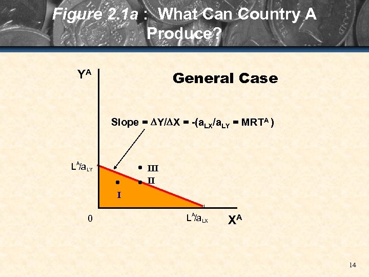
Figure 2. 1 a : What Can Country A Produce? General Case YA Slope = Y/ X = -(a. LX/a. LY = MRTA ) LA/a. LY III II I 0 LA/a. LX XA 14

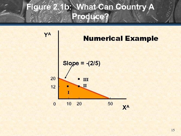
Figure 2. 1 b: What Can Country A Produce? YA Numerical Example Slope = -(2/5) 20 III II 12 I 0 10 20 50 XA 15

Production in Autarky • Numerical example (Figure 2. 1 b): – Country A can use its labor endowment (LA = 100) to produce LA/a. LX (100/2 = 50) units of good X, and LA/a. LY (100/5 = 20) units of good Y. • The slope of the frontier (-[a. LX/a. LY], or – 2/5 gives the opportunity cost of good X, or the rate at which good X can be “transformed” into good Y. – Opportunity cost of good X • Number of units of good Y forgone to produce an additional unit of good X. 16

Production in Autarky • Marginal rate of transformation (MRT) – Rate at which good X can be “transformed” into good Y by transferring labor out of the X industry and into the Y industry. • Ricardian model implies the PPF is a straight line. – Model sometimes referred to as a constant-cost model. • Production opportunity set – All possible combinations of X and Y a country could produce. 17

Production in Autarky • Consumption opportunity set – All possible combinations of X and Y its residents could consume. • Production and consumption opportunity sets coincide in autarky. 18

Consumption in Autarky • Assumptions: – Level of satisfaction or utility of residents depends on quantities of goods X and Y available for consumption. – Production/consumption decision is made in such a way as to maximize utility. – Graphical technique of indifference curves show all different combinations of goods X and Y that result in a given level of utility. 19

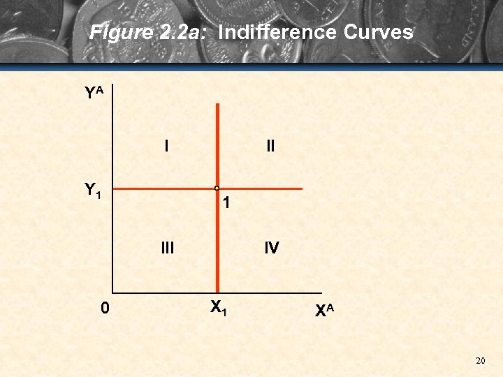
Figure 2. 2 a: Indifference Curves YA I Y 1 III 0 IV X 1 XA 20

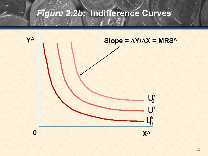
Figure 2. 2 b: Indifference Curves YA 0 Slope = Y/ X = MRSA XA 21

Consumption in Autarky • Four basic properties of indifference curves: – 1. Are downward sloping. • See Fig. 2. 2 a: Areas I and IV represent the possibilities of substituting more of one good for less of the other with no change in overall utility. – The fact that residents must be compensated for the loss of one good by more of the other good to maintain the same level of utility implies that indifference curves must be downward sloping. 22

Consumption in Autarky • Four basic properties of indifference curves: – 2. Must be convex. • Slope represents the rate at which residents are willing to trade off consumption of the two goods (called Marginal Rate of Substitution [MRS]). • As more X and less Y is consumed (moving down the indifference curve), good Y becomes more highly valued relative to good X. 23

Consumption in Autarky • Four basic properties of indifference curves: – 3. Indifference curves never intersect. • Each point (combination of goods X and Y, lies on one, and only one, indifference curve. – 4. Higher indifference curves represent higher levels off utility. • Are preferred to lower indifference curves. 24

Consumption in Autarky • Community Indifference Curves: – Represent tastes of a country’s residents as a group. – More complicated than indifference curves, which represent the tastes of an individual. • Communities present Income Distribution problem: Range of preferences and degrees of wealth. • Increased availability of goods always raises Potential Utility. – Income distribution determines utility increases or decreases. 25

Equilibrium in Autarky • In autarky, production/consumption decisions are made by maximizing utility subject to constraint imposed by PPF. – In Fig. 2. 3, Point A* puts residents on indifference curve U 1 representing the highest level of satisfaction attainable given the country’s resource endowment (LA) and available technology (a. LX and a. LY). • Point A* = country’s autarky equilibrium (allocation of resources which produces highest level of utility for country’s residents). 26

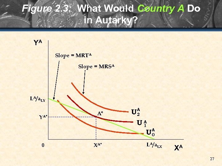
Figure 2. 3: What Would Country A Do in Autarky? YA Slope = MRTA Slope = MRSA LA/a. LY YA* 0 A* XA* A U 2 UA 1 A U 0 LA/a. LX XA 27

Equilibrium in Autarky • At Point A* the marginal rate of transformation equals the marginal rate of substitution. – Common slope of production possibilities and indifference curve represents the opportunity cost of good X expressed in terms of good Y. 28

Equilibrium in Autarky • Due to perfect competition, the relative price of each good equals its opportunity cost. – Therefore, the slope of the production possibilities frontier can be identified with the relative price of good X in country A, or (PX/PY)A. • This relative price is autarky relative price of good X in country A. 29

Equilibrium in Autarky • The wage rate in country A must include these 3 assumptions: – Labor comprises the only inputs. – Price of each good equals its marginal cost (due to perfect competition). – Wage rate must be equal in the two industries. 30

Ricardian World with Trade • Country B is a potential trading partner for Country A. – B’s autarky situation resembles A’s. • However, there is no reason to believe that both countries will have identical quantities of labor available or use the same technology. – If technologies differ, then the production possibilities frontiers will generally have different slopes – these differences form the basis for mutually beneficial trade. • Also, no reason to expect preferences of B’s residents to be same as those of country A’s. 31

Ricardian World with Trade • Figure 2. 4 shows B’s autarky equilibrium at B*. – To demonstrate the potential of international trade for improving the welfare of residents of A and B, it is important to show that the allocation of resources at A* and B* does not maximize total world output. • Moving away from A* and B* allows increased production of one good without decreasing production of the other. – Adam Smith first demonstrated this fundamental result using concept of absolute advantage. 32

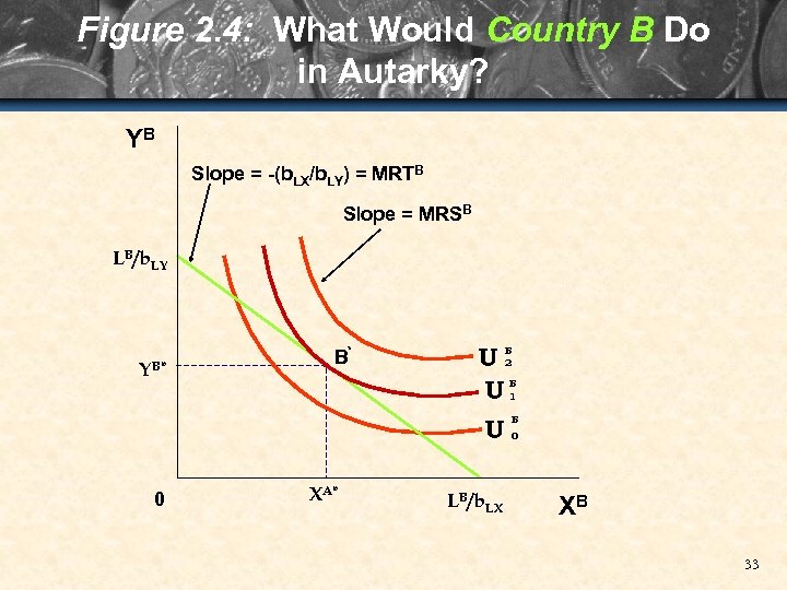
Figure 2. 4: What Would Country B Do in Autarky? YB Slope = -(b. LX/b. LY) = MRTB Slope = MRSB LB/b. LY YB* 0 B* XA* U U U LB/b. LX B 2 B 1 B 0 XB 33

Adam Smith and Absolute Advantage • Country A has absolute advantage in production of good X if a. LX < b. LX. – It takes fewer units of labor to produce a unit of good X in country A than in B. • Smith asserted that international trade between two countries would be mutually beneficial whenever one country had an absolute advantage in production of one good and the other country had an absolute advantage in production of the other good. – It would benefit each country to specialize in producing goods in which it had absolute advantage and import goods in which it had absolute disadvantage. 34

Adam Smith and Absolute Advantage • Smith’s main contribution was the concept that trade is not a zero-sum game. – Mutually beneficial trade required each country to have an absolute advantage in one of the goods. • This requirement ruled out many potential trading relationships in which one of the countries had an absolute advantage in both goods. 35

David Ricardo and Comparative Advantage • Ricardo demonstrated that mutually beneficial trade is possible even if one potential trading partner has absolute advantage in production of both goods. – Used concept of Comparative Advantage. • Country A has comparative advantage in production of good X if (a. LX/a. LY) < (b. LX/b. LY). – Would be beneficial for a country to specialize in the production of the good in which it has a comparative advantage and to trade for the good in which it has a comparative disadvantage. 36

David Ricardo and Comparative Advantage – This specialization makes both countries potentially better off by expanding their consumption opportunity sets. • Specialization and trade allow a country’s consumption opportunity set to expand beyond its production opportunity set. – In Figures 2. 5 a and 2. 5 b, at points AP and BP, the total quantity of X and Y produced is maximized given the available resources and technology. • Additional units of either good can be produced only by decreasing production of the other. 37

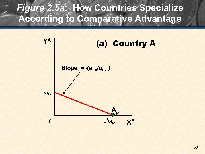
Figure 2. 5 a: How Countries Specialize According to Comparative Advantage YA (a) Country A Slope = -(a. LX/a. LY ) LA/a. LY Ap 0 LA/a. LX XA 38

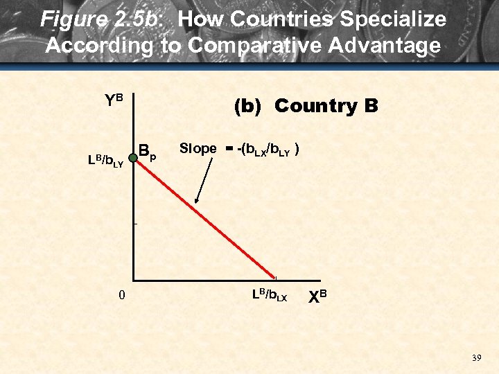
Figure 2. 5 b: How Countries Specialize According to Comparative Advantage (b) Country B YB LB/b LY 0 Bp Slope = -(b. LX/b. LY ) LB/b. LX XB 39

International Equilibrium with Trade • Once both countries have opened trade and specialized production according to comparative advantage, equilibrium price ratio at which trade occurs (written as [PX/PY]tt and called the Terms of Trade) must lie between the two countries’ autarky price ratios. – A country would never trade voluntarily at international terms of trade less favorable than its own autarky price ratio. 40

International Equilibrium with Trade • Figure 2. 6 a – For country A to trade voluntarily with country B, the international terms of trade must be more favorable to A than are its own production possibilities or domestic opportunity costs. • For any terms of trade represented as a line from point AP that is steeper than the production possibilities frontier, country A can obtain more units of Y through trade than production. 41

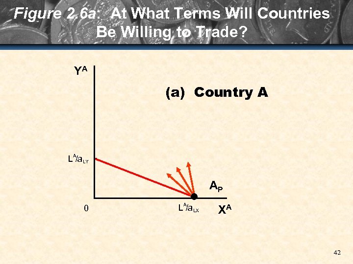
Figure 2. 6 a: At What Terms Will Countries Be Willing to Trade? YA (a) Country A LA/a. LY AP 0 LA/a. LX XA 42

International Equilibrium with Trade • Figure 2. 6 b – Because B can get one unit of X through domestic production by forgoing b. LX/b. LY units of Y, B will trade voluntarily only if it can obtain a unit of X for fewer than b. LX/b. LY units of Y. • Therefore, all terms of trade at which B would willingly trade are represented by lines from point BP that are flatter than B’s production possibilities frontier. 43

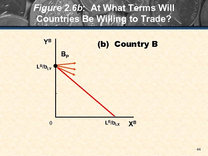
Figure 2. 6 b: At What Terms Will Countries Be Willing to Trade? (b) Country B YB BP LB/b. LY 0 LB/b. LX XB 44

International Equilibrium with Trade • International terms of trade must satisfy one additional condition: – Equilibrium terms of trade also must be the Market-Clearing Price for the two goods. • Quantity of X that A wants to export at the terms of trade must equal the quantity of X that B wants to import at the same terms of trade. – Similarly with good Y. 45

International Equilibrium with Trade • Each country takes advantage of new opportunities by locating at the point of tangency of the highest possible indifference curve and the terms-of-trade line. – In Figures 2. 7 and 2. 8, A produces at point AP and consumes at AC, and B produces at BP and consumes at BC. • Shaded triangles (Trade Triangles) summarize each country’s imports and exports, as well as the terms of trade. – Wages rise in both countries with the opening of trade. 46

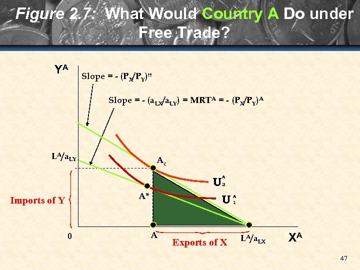
Figure 2. 7: What Would Country A Do under Free Trade? YA Slope = - (PX/PY)tt Slope = - (a. LX/a. LY) = MRTA = - (PX/PY)A LA/a. LY Ac U A 2 A* Imports of Y 0 U A Exports of X A 1 LA/a. LX XA 47

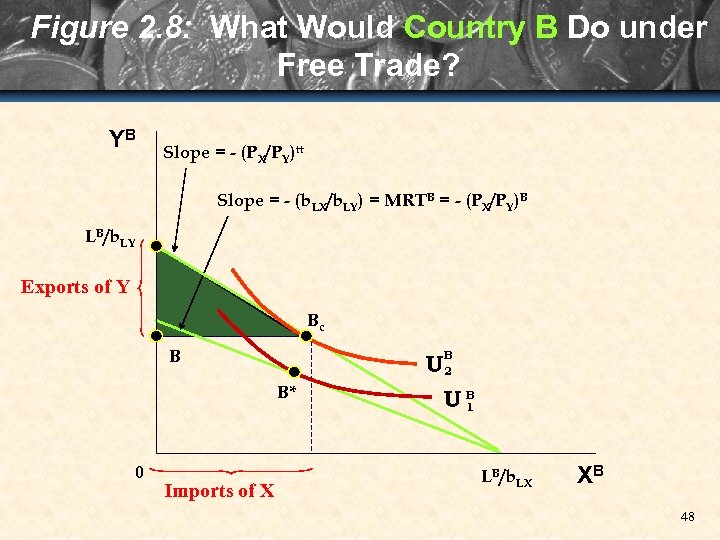
Figure 2. 8: What Would Country B Do under Free Trade? YB Slope = - (PX/PY)tt Slope = - (b. LX/b. LY) = MRTB = - (PX/PY)B LB/b. LY Exports of Y Bc B B 2 U B* 0 Imports of X UB 1 LB/b. LX XB 48

Gains from Trade • Gains from Exchange, one portion of gains from trade, comes from allowing unrestricted exchange of goods between countries without altering the autarky production patterns. – Rather than consuming the goods produced domestically, residents of A exchange with residents of B. – A willing to export X at any relative higher than (PX/PY)A, its autarky price 49

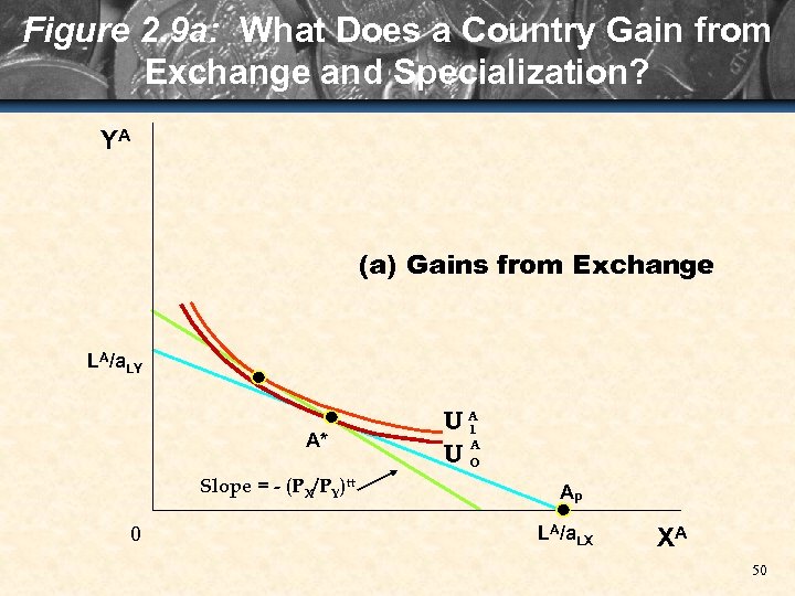
Figure 2. 9 a: What Does a Country Gain from Exchange and Specialization? YA (a) Gains from Exchange LA/a. LY A* Slope = - (PX/PY)tt 0 UA 1 A U 0 AP LA/a. LX XA 50

Gains from Trade • Remainder of gains from trade come from production specialization according to comparative advantage – called Gains from Specialization. – With the possibility of trade, countries no longer choose to produce the same combination of goods they did in autarky. 51

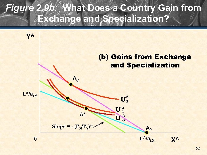
Figure 2. 9 b: What Does a Country Gain from Exchange and Specialization? YA (b) Gains from Exchange and Specialization AC LA/a. LY A U 2 A* Slope = - (PX/PY)tt 0 UA 1 A U 0 AP LA/a. LX XA 52

Demand Supply in Autarky • In autarky, the market for each good in each country is isolated from the market for the same good in the other country. – Therefore, there are four markets (one for each of the two goods in each of the two countries) represented by Figures 2. 10 a through 2. 10 d. • In each of the 4 markets, the interaction of domestic demand domestic supply determines the good’s autarky relative price. 53

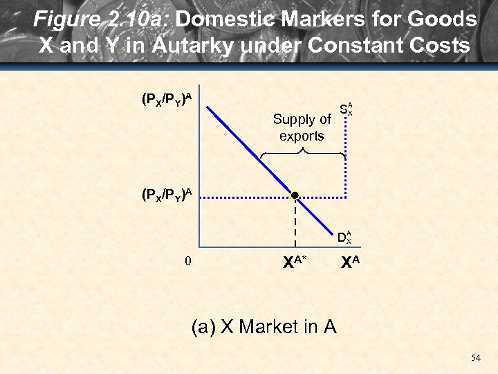
Figure 2. 10 a: Domestic Markers for Goods X and Y in Autarky under Constant Costs (PX/PY)A Supply of exports SA X (PX/PY)A DA X 0 XA* XA (a) X Market in A 54

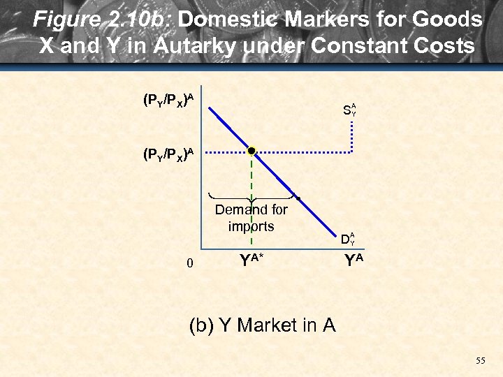
Figure 2. 10 b: Domestic Markers for Goods X and Y in Autarky under Constant Costs (PY/PX)A SA Y (PY/PX)A Demand for imports 0 YA* DA Y YA (b) Y Market in A 55

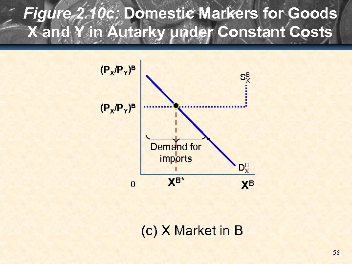
Figure 2. 10 c: Domestic Markers for Goods X and Y in Autarky under Constant Costs (PX/PY)B SB X (PX/PY)B Demand for imports 0 XB* DB X XB (c) X Market in B 56

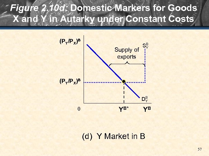
Figure 2. 10 d: Domestic Markers for Goods X and Y in Autarky under Constant Costs (PY/PX)B Supply of exports SB Y (PY/PX)B DB Y 0 YB* YB (d) Y Market in B 57

Demand Supply with Trade • The opening of trade allows countries A and B to participate in a common international market for each good. – Figure 2. 11 a represents the international market for good X. – Figure 2. 11 b represents the international market for good Y. 58

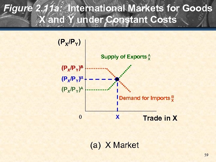
Figure 2. 11 a: International Markets for Goods X and Y under Constant Costs (PX/PY) Supply of Exports A X (PX/PY)B (PX/PY)tt (PX/PY)A Demand for Imports B X 0 Xtt Trade in X (a) X Market 59

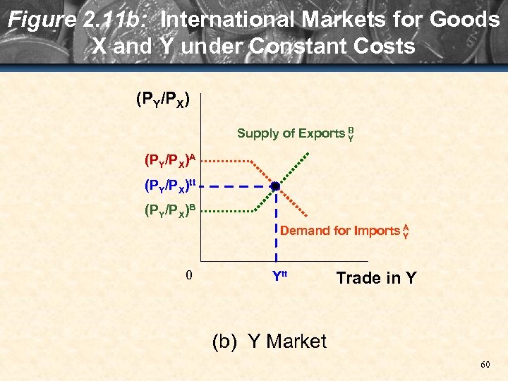
Figure 2. 11 b: International Markets for Goods X and Y under Constant Costs (PY/PX) Supply of Exports B Y (PY/PX)A (PY/PX)tt (PY/PX)B Demand for Imports A Y 0 Ytt Trade in Y (b) Y Market 60

Demand Supply with Trade • Each country is willing to import its good of comparative disadvantage at prices below its autarky price. – At each price, the quantity demanded of imports equals the difference between quantity demanded and quantity produced domestically. • Each country also is willing to export its good of comparative advantage at prices above its autarky price. – At each price, the quantity supplied of exports equals the difference between quantity supplied and quantity demanded domestically. 61

Note for Case 1: Can the Ricardian Model Really Explain Trade? • Figure 2. 12 compares relative labor productivity with export performance. – The empirical results clearly support the Ricardian idea that a country tends to export goods in which its labor is relatively productive. 62

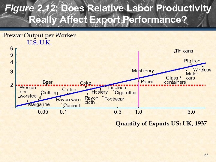
Figure 2. 12: Does Relative Labor Productivity Really Affect Export Performance? Prewar Output per Worker U. S. : U. K. 6 5 4 Tin cans Pig iron Machinery 3 2 1 Beer Paper Coke Wireless Motor cars Glass containers Woolen Linoleum Cotton and Hosiery Cigarettes Clothing worsted Rayon yarn Rayon Footwear cloth Margarine Cement 0. 05 0. 1 0. 5 1. 0 5. 0 Quantity of Exports US: UK, 1937 63

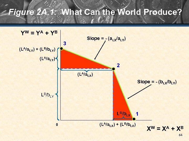
Figure 2 A. 1: What Can the World Produce? YW = Y A + Y B 3 Slope = - (a. LX/a. LY) (LA/a. LY) + (LB/b. LY) (LA/a. LY) 2 (LA/a. LX) Slope = - (b. LX/b. LY) LB/b. LY LB/b. LX 0 (LA/a. LX) + (LB/b. LX) 1 XW = X A + X B 64

Key Terms in Chapter 2 • Mercantilism • Zero-sum game • Specie-flow mechanism • Perfect competition • Marginal cost • Autarky • Production possibilities frontier 65

Key Terms in Chapter 2 • Input coefficient • Opportunity cost • Marginal rate of transformation (MRT) • Ricardian model • Constant-cost model • Production opportunity set • Consumption opportunity set 66

Key Terms in Chapter 2 • • • Utility Indifference curve Marginal rate of substitution (MRS) Community indifference curves Income distribution Potential utility Autarky equilibrium Autarky relative price Absolute advantage 67

Key Terms in Chapter 2 • • Absolute disadvantage Comparative advantage Terms of trade Market-clearing price Trade triangles Gains from exchange Gains from specialization 68