Chapter Three Preferences Rationality in Economics


varian_chapter03_preferences_mod.ppt
- Размер: 248 Кб
- Количество слайдов: 71
Описание презентации Chapter Three Preferences Rationality in Economics по слайдам
 Chapter Three Preferences
 Rationality in Economics Behavioral Postulate : A decisionmaker always chooses its most preferred alternative from its set of available alternatives. So to model choice we must model decisionmakers’ preferences.
 Consumption bundle – object of consumer choice. Consumption bundle – complete list of goods and services, the consumer can choose from. When, where and under what circumstances matter
 Consumption bundle X consists of x 1 , x 2 , …. Xn goods and services For simplicty assume – X consists of only 2 goods: x 1 , x 2 ,
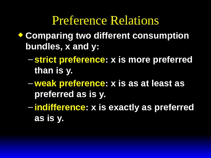
 Preference Relations Comparing two different consumption bundles, x and y: – strict preference : x is more preferred than is y. – weak preference : x is as at least as preferred as is y. – indifference : x is exactly as preferred as is y.
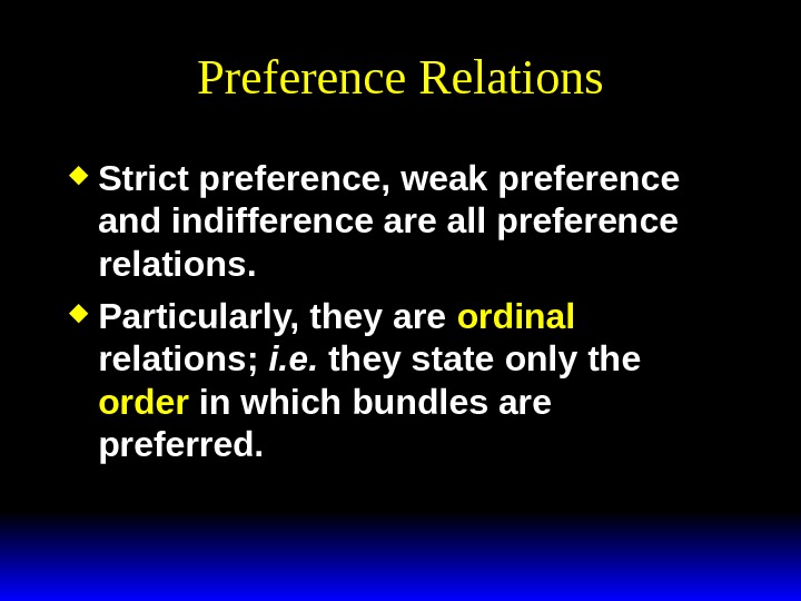
 Preference Relations Strict preference, weak preference and indifference are all preference relations. Particularly, they are ordinal relations; i. e. they state only the order in which bundles are preferred.
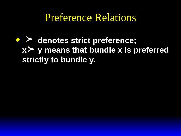
 Preference Relations denotes strict preference; x y means that bundle x is preferred strictly to bundle y.
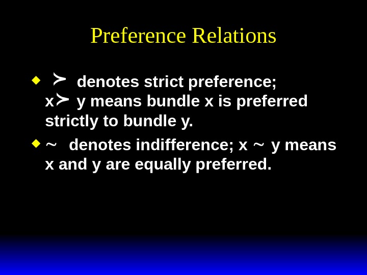
 Preference Relations denotes strict preference; x y means bundle x is preferred strictly to bundle y. denotes indifference; x y means x and y are equally preferred.
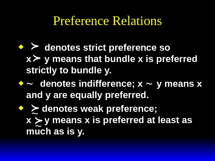
 Preference Relations denotes strict preference so x y means that bundle x is preferred strictly to bundle y. denotes indifference; x y means x and y are equally preferred. denotes weak preference; x y means x is preferred at least as much as is y. ~ ~
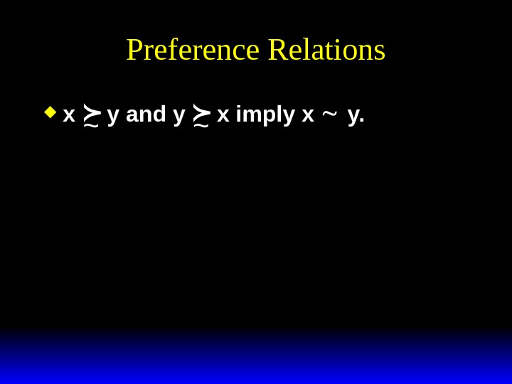
 Preference Relations x y and y x imply x y. ~ ~
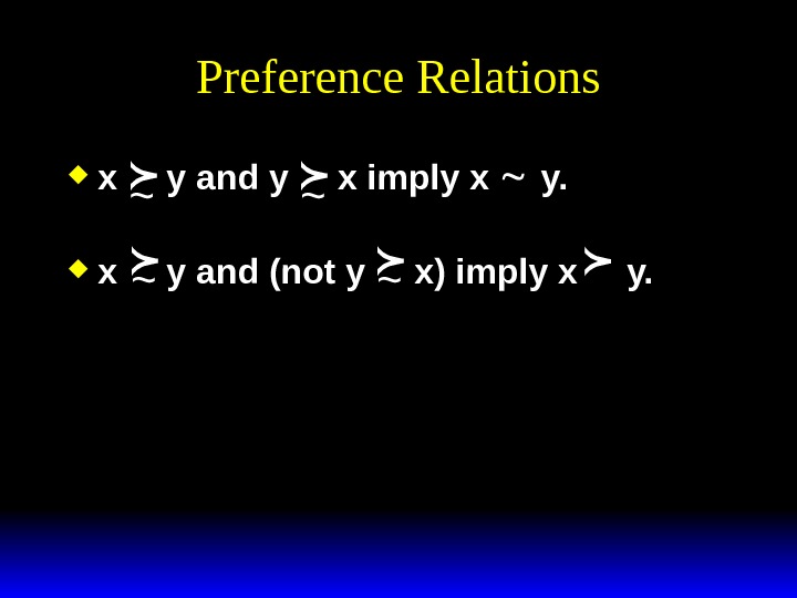
 Preference Relations x y and y x imply x y. x y and (not y x) imply x y. ~ ~
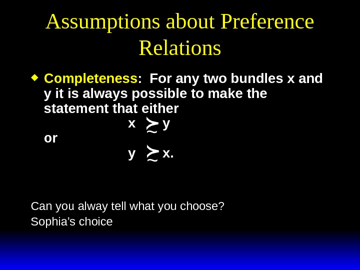
 Assumptions about Preference Relations Completeness : For any two bundles x and y it is always possible to make the statement that either x y or y x. Can you alway tell what you choose? Sophia’s choice ~ ~
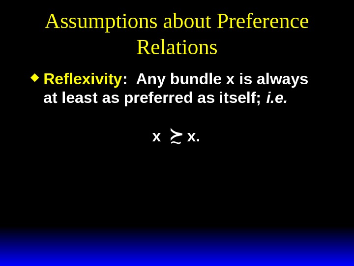
 Assumptions about Preference Relations Reflexivity : Any bundle x is always at least as preferred as itself; i. e. x x. ~
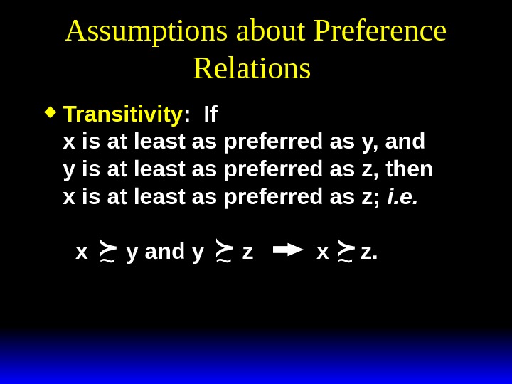
 Assumptions about Preference Relations Transitivity : If x is at least as preferred as y, and y is at least as preferred as z, then x is at least as preferred as z; i. e. x y and y z x z. ~ ~ ~
 Transitivity –an experiment Imagine you are hungry. During the break you may have ……. What would you choose? Write the first letter in the table given to you and bend the row, so that you can not see the previous choices
 Transitivity –an experiment 1. Apple vs. Banana
 Transitivity –an experiment 2. Banana vs. Cake
 Transitivity –an experiment 3. Cake vs. Sandwich with Ham
 Transitivity –an experiment 4. Sandwich with Ham vs. Sandwich with Cheese
 Transitivity –an experiment 5. Apple vs. Cake
 Transitivity –an experiment 6. Apple vs. Sandwich with Cheese
 Transitivity –an experiment 7. Apple vs. Sandwich with Ham
 Transitivity –an experiment 8. Banana vs. Sandwich with Ham
 Transitivity –an experiment 9. Banana vs. Sandwich with Cheese
 Transitivity –an experiment 10. Cake vs. Sandwich with Cheese
 Assumptions about Preference Relations Transitivity is a hypothesis about people’s choice behaviour – not a statement of pure logic! We have to assume preferences are transitive to have a theory of how people make best choices
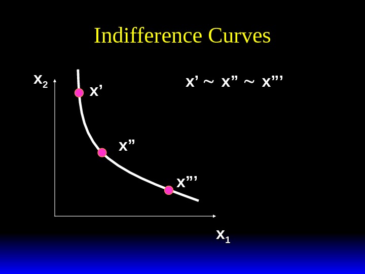
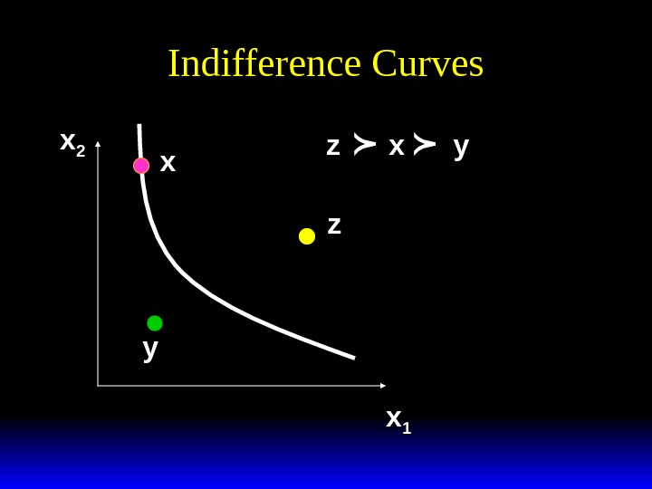
 Indifference Curves Take a reference bundle x’. The set of all bundles equally preferred to x’ is the indifference curve containing x’ ; the set of all bundles y x’. Since an indifference “curve” is not always a curve a better name might be an indifference “set”.
 Indifference Curves xx 22 xx 11 x”x” x”’x”’ x’ x’ x” x” x”’ x’
 Indifference Curves xx 22 xx 11 zz xx yy x y z
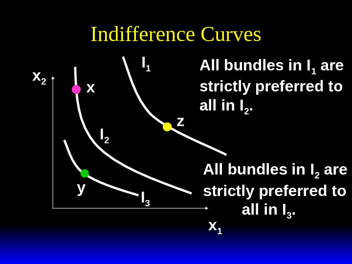
 Indifference Curves x 2 x 1 x All bundles in I 1 are strictly preferred to all in I 2. y z All bundles in I 2 are strictly preferred to all in I 3. I 1 I 2 I
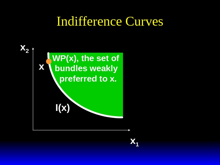
 Indifference Curves x 2 x 1 I(x’)x I(x)WP(x), the set of bundles weakly preferred to x.
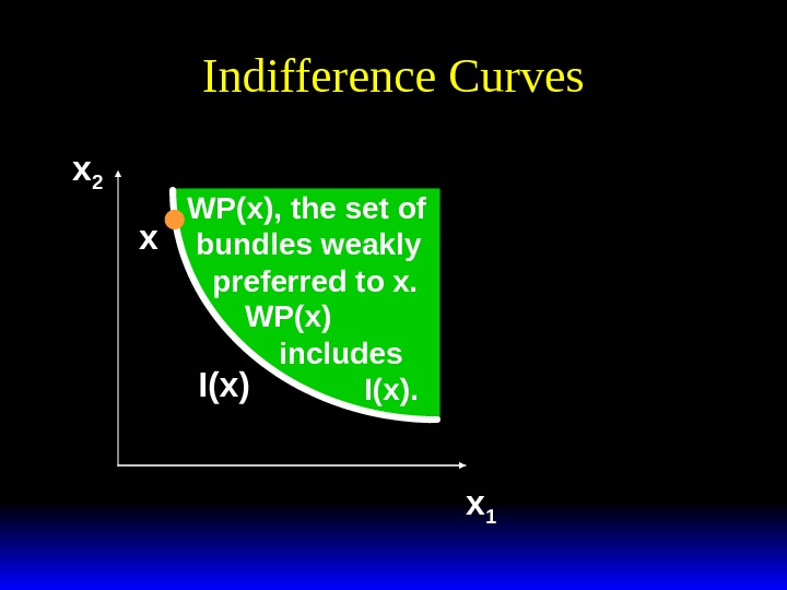
 Indifference Curves x 2 x 1 WP(x), the set of bundles weakly preferred to x. WP(x) includes I(x). x I(x)
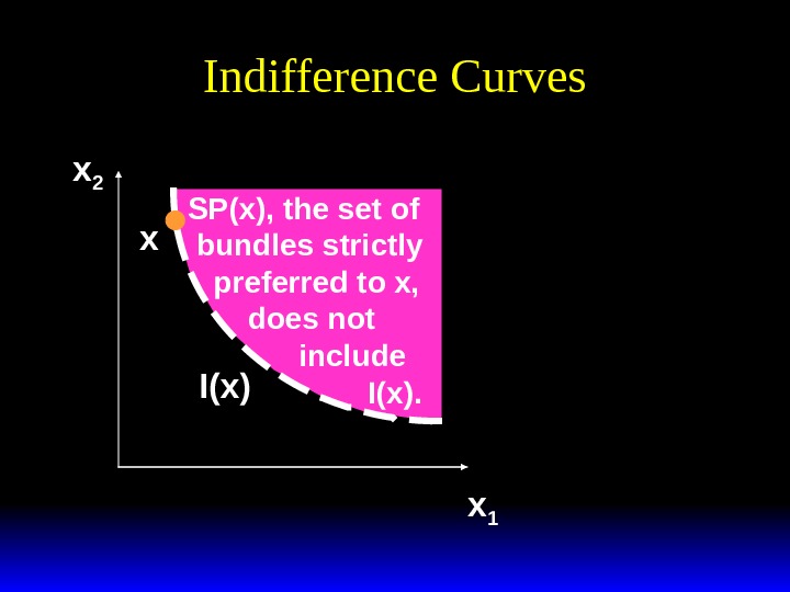
 Indifference Curves x 2 x 1 SP(x), the set of bundles strictly preferred to x, does not include I(x). x I(x)
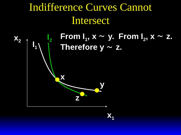
 Indifference Curves Cannot Intersect xx 22 xx 11 xx yy zz. II 11 I 2 From I 11 , x y. From I 22 , x z. z. Therefore y z. z.
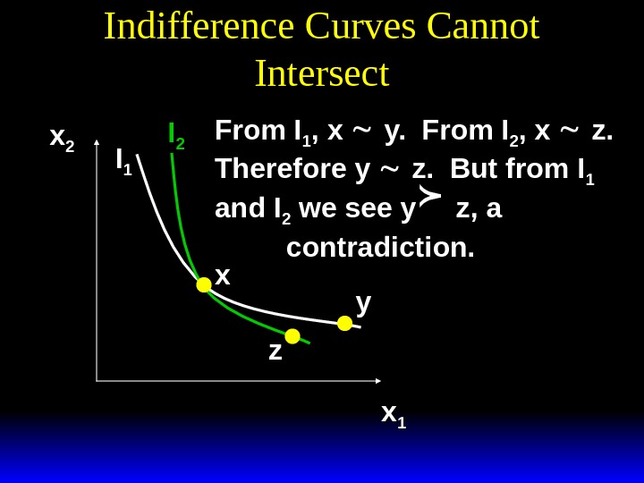
 Indifference Curves Cannot Intersect xx 22 xx 11 xx yy zz. II 11 I 2 From I 11 , x y. From I 22 , x z. z. Therefore y z. But from I 11 and I 22 we see y z, a contradiction.
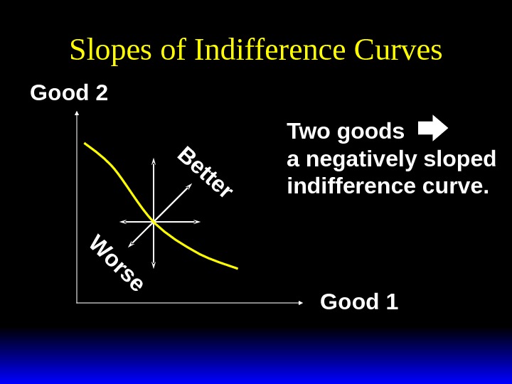
 Slopes of Indifference Curves When more of a commodity is always preferred, the commodity is a good. If every commodity is a good then indifference curves are negatively sloped.
 Slopes of Indifference Curves. B e tte r W o rs e Good 2 Good 1 Two goods a negatively sloped indifference curve.
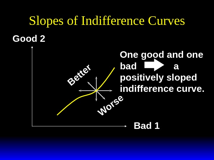
 Slopes of Indifference Curves If less of a commodity is always preferred then the commodity is a bad.
 Slopes of Indifference Curves. B e tte r W o rs e Good 2 Bad 1 One good and one bad a positively sloped indifference curve.
 Slopes of Indifference Curves If the consumer doesn’t care about a good then this good is a neutral good.
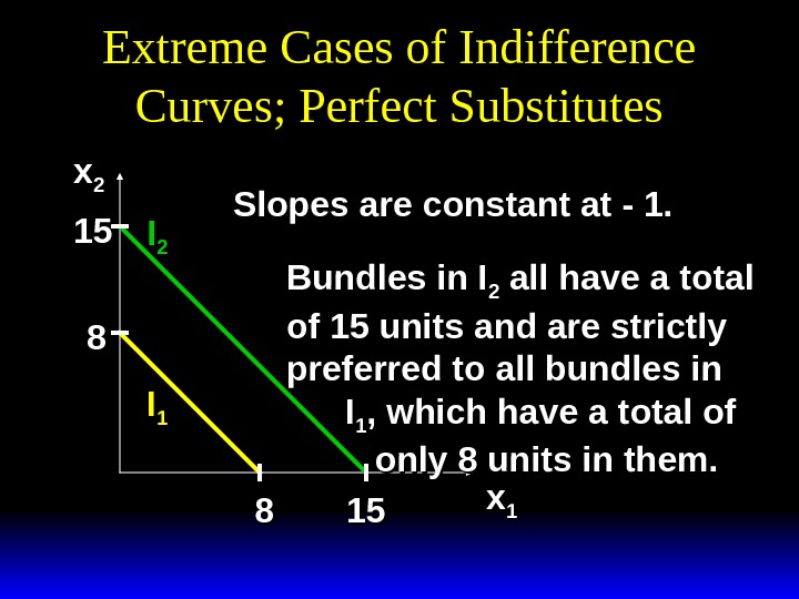
 Extreme Cases of Indifference Curves; Perfect Substitutes If a consumer always regards units of commodities 1 and 2 as equivalent, then the commodities are perfect substitutes and only the total amount of the two commodities in bundles determines their preference rank-order.
 Extreme Cases of Indifference Curves; Perfect Substitutes xx 22 xx 11 8888 1515 Slopes are constant at — 1. I 2 I 1 Bundles in I 22 all have a total of 15 units and are strictly preferred to all bundles in I I 11 , which have a total of only 8 units in them.
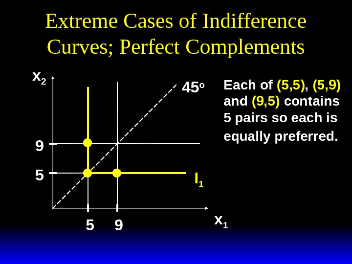
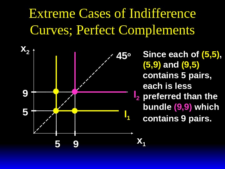
 Extreme Cases of Indifference Curves; Perfect Complements If a consumer always consumes commodities 1 and 2 in fixed proportion (e. g. one-to-one), then the commodities are perfect complements and only the number of pairs of units of the two commodities determines the preference rank-order of bundles.
 Extreme Cases of Indifference Curves; Perfect Complements xx 22 xx 11 I 14545 oo 55 99 Each of (5, 5) , (5, 9) and (9, 5) contains 5 pairs so each is equally preferred.
 Extreme Cases of Indifference Curves; Perfect Complements xx 22 xx 11 I 2 I 14545 oo 55 99 Since each of (5, 5) , (5, 9) and (9, 5) contains 5 pairs, each is less preferred than the bundle (9, 9) which contains 9 pairs.
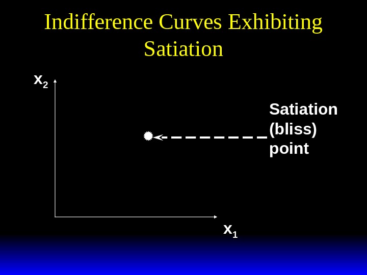
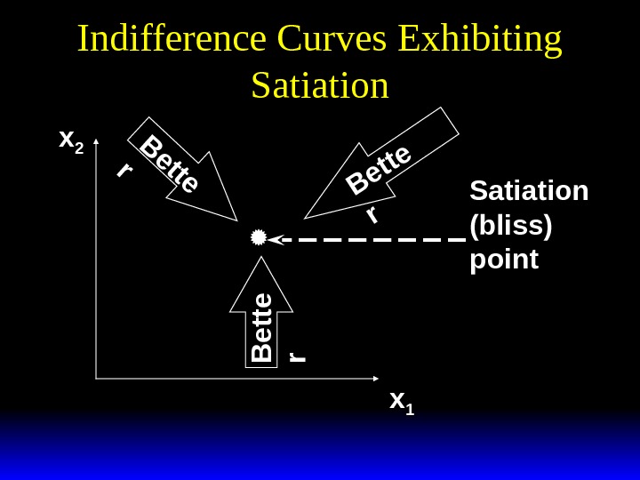
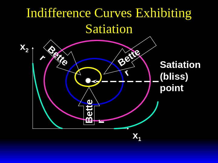
 Preferences Exhibiting Satiation A bundle strictly preferred to any other is a satiation point or a bliss point. What do indifference curves look like for preferences exhibiting satiation?
 Indifference Curves Exhibiting Satiation xx 22 xx 11 Satiation (bliss) point
 Indifference Curves Exhibiting Satiation xx 22 xx 11 B ette rr B e t t e rr Satiation (bliss) point
 Indifference Curves Exhibiting Satiation xx 22 xx 11 B ette rr B e t t e rr Satiation (bliss) point
 Indifference Curves for Discrete Commodities A commodity is infinitely divisible if it can be acquired in any quantity; e. g. water or cheese. A commodity is discrete if it comes in unit lumps of 1, 2, 3, … and so on; e. g. aircraft, ships and refrigerators , egs.
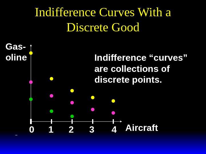
 Indifference Curves for Discrete Commodities Suppose commodity 2 is an infinitely divisible good (gasoline) while commodity 1 is a discrete good (aircraft). What do indifference “curves” look like?
 Indifference Curves With a Discrete Good Gas- oline Aircraft 00 11 22 3 44 Indifference “curves” are collections of discrete points.
 Well-Behaved Preferences A preference relation is “ well-behaved ” if it is – monotonic and convex. Monotonicity : More of any commodity is always preferred ( i. e. no satiation and every commodity is a good).
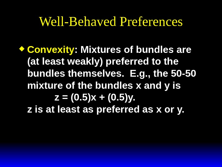
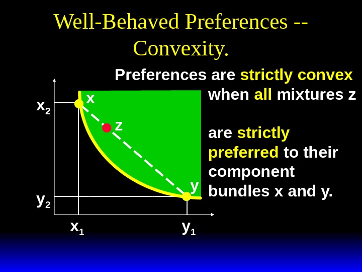
 Well-Behaved Preferences Convexity : Mixtures of bundles are (at least weakly) preferred to the bundles themselves. E. g. , the 50 -50 mixture of the bundles x and y is z = (0. 5)x + (0. 5)y. z is at least as preferred as x or y.
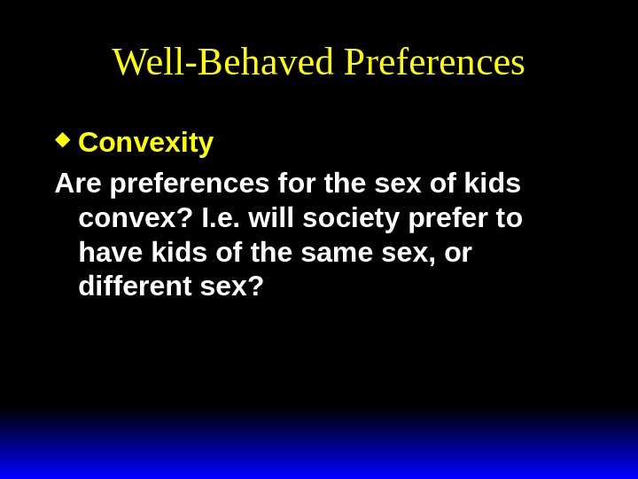
 Well-Behaved Preferences Convexity Are preferences for the sex of kids convex? I. e. will society prefer to have kids of the same sex, or different sex?
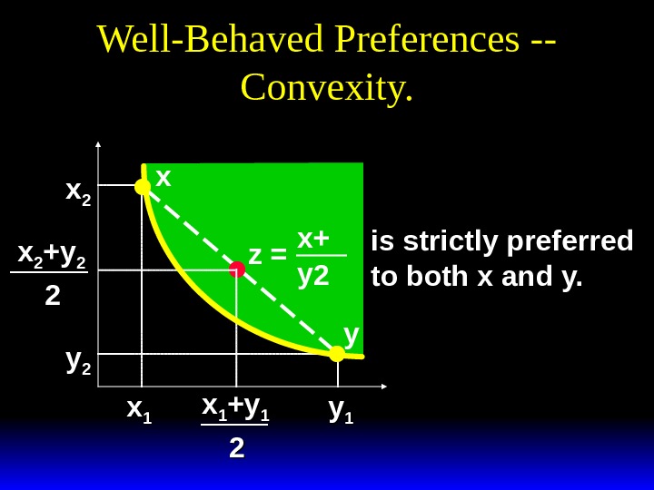
 Well-Behaved Preferences — Convexity. xx 22 yy 22 xx 22 +y+y 22 22 xx 11 yy 11 xx 11 +y+y 11 22 x yz = x+ y 2 is strictly preferred to both x and y.
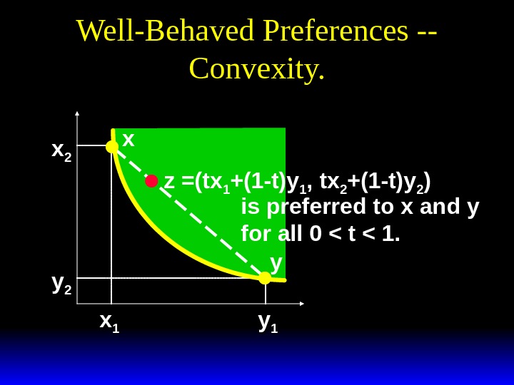
 Well-Behaved Preferences — Convexity. xx 22 yy 22 xx 11 yy 11 x yz =(tx 1 +(1 -t)y 1 , tx 2 +(1 -t)y 2 ) is preferred to x and y for all 0 < t < 1.
 Well-Behaved Preferences — Convexity. xx 22 yy 22 xx 11 yy 11 x y. Preferences are strictly convex when all mixtures z are strictly preferred to their component bundles x and y. z
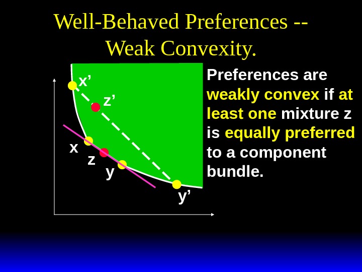
 Well-Behaved Preferences — Weak Convexity. x’ y’z’ Preferences are weakly convex if at least one mixture z is equally preferred to a component bundle. x z y
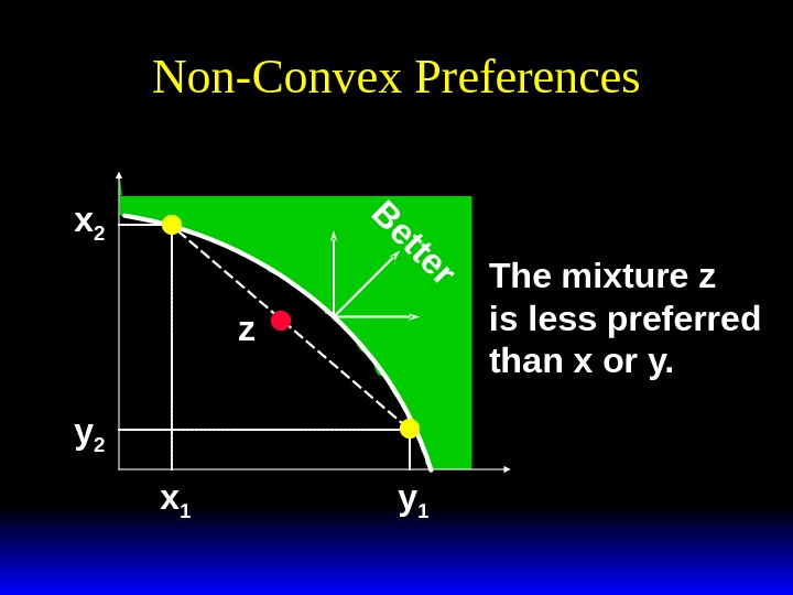
 Non-Convex Preferences xx 22 yy 22 xx 11 yy 11 zz. B e tte r The mixture z is less preferred than x or y.
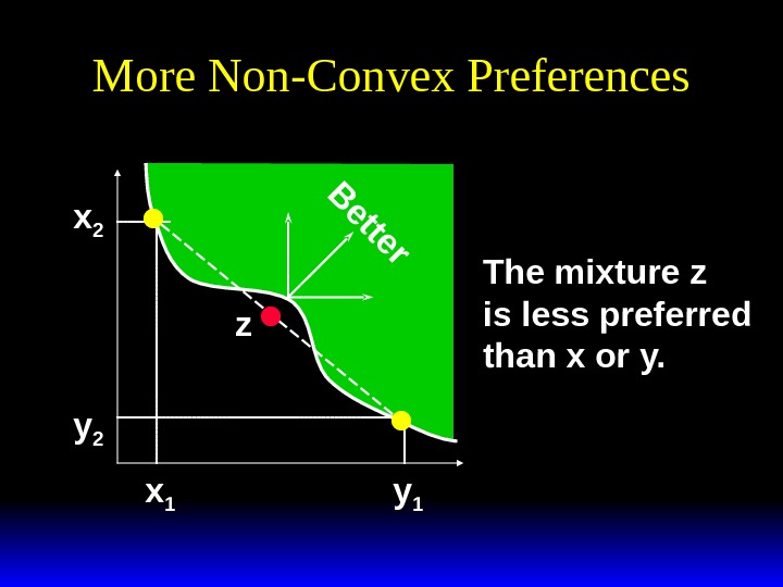
 More Non-Convex Preferences xx 22 yy 22 xx 11 yy 11 zz. B e tte r The mixture z is less preferred than x or y.
 Slopes of Indifference Curves The slope of an indifference curve is its marginal rate-of-substitution (MRS). How can a MRS be calculated?
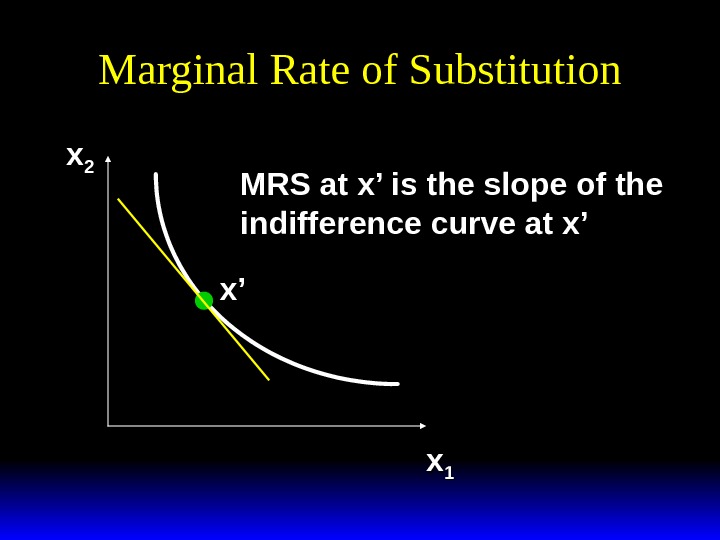
 Marginal Rate of Substitution xx 22 xx 11 x’x’ MRS at x’ is the slope of the indifference curve at x’
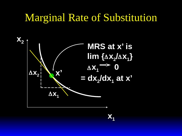
 Marginal Rate of Substitution xx 22 xx 11 MRS at x’ is lim { xx 22 // xx 11 }} xx 11 0 0 = dx 22 /dx/dx 11 at x’ xx 22 xx 11 x’x’
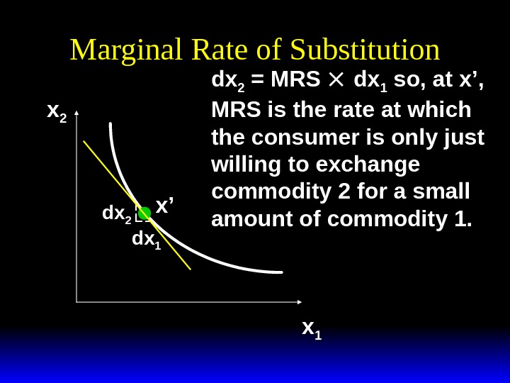
 Marginal Rate of Substitution xx 22 x 1 dxdx 22 dxdx 11 dxdx 22 = MRS dx dx 11 so, at x’, MRS is the rate at which the consumer is only just willing to exchange commodity 2 for a small amount of commodity 1. x’x’
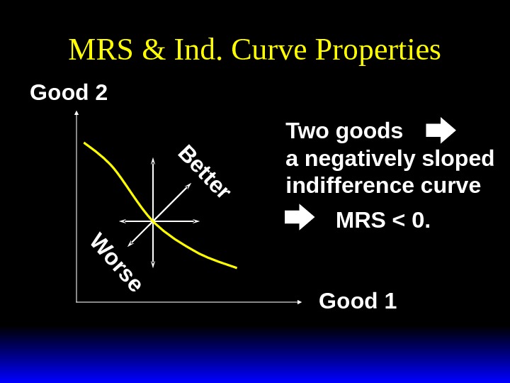
 MRS & Ind. Curve Properties. B e tte r W o rs e Good 2 Good 1 Two goods a negatively sloped indifference curve MRS < 0.
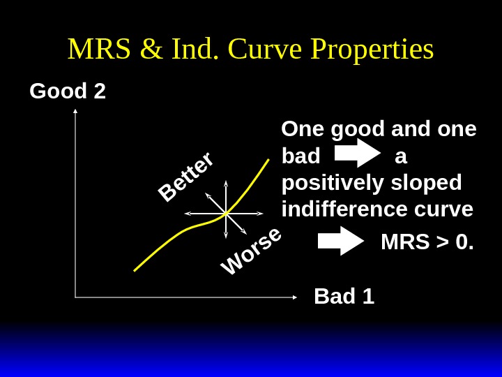
 MRS & Ind. Curve Properties. B e tte r W o rs e Good 2 Bad 1 One good and one bad a positively sloped indifference curve MRS > 0.
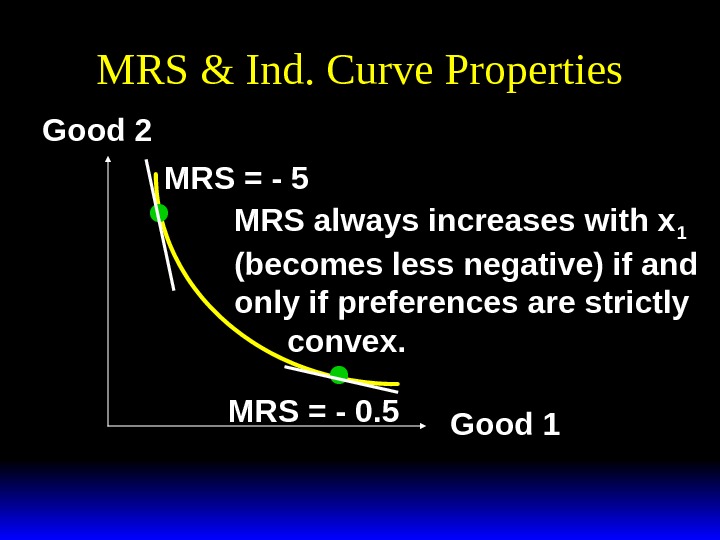
 MRS & Ind. Curve Properties Good 2 Good 1 MRS = — 5 MRS = — 0. 5 MRS always increases with x 11 (becomes less negative) if and only if preferences are strictly convex.
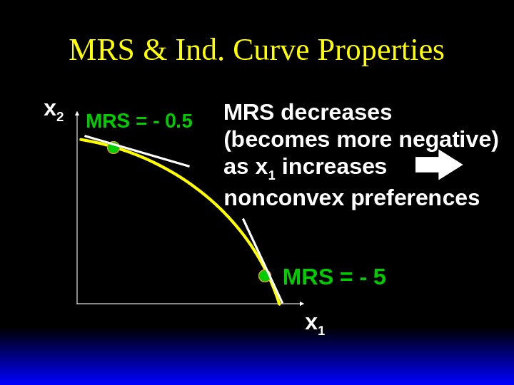
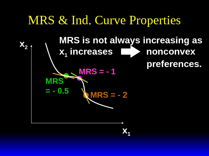
 MRS & Ind. Curve Properties xx 11 xx 22 MRS = — 0. 5 MRS = — 5 MRS decreases (becomes more negative) as x 11 increases nonconvex preferences
 MRS & Ind. Curve Properties xx 22 xx 11 MRS = — 0. 5 MRS = — 1 MRS = — 2 MRS is not always increasing as xx 11 increases nonconvex preferences.
 Marginal Rate of Substitution MRS is sometimes called marginal willingness to pay. This happens when good x 2 represents „all other goods” and is measured in dollars. Remember it is marginal and it is willingness

