Varian_Chapter06_Demand_mod.ppt
- Количество слайдов: 123
 Chapter Six Demand
 Properties of Demand Functions u Comparative statics analysis of ordinary demand functions -- the study of how ordinary demands x 1*(p 1, p 2, y) and x 2*(p 1, p 2, y) change as prices p 1, p 2 and income y change.
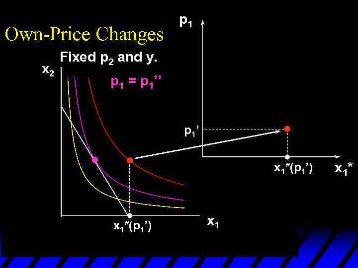
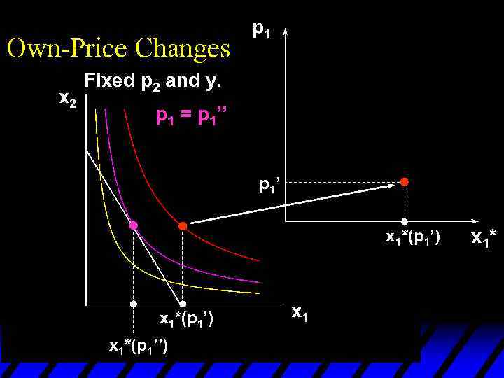
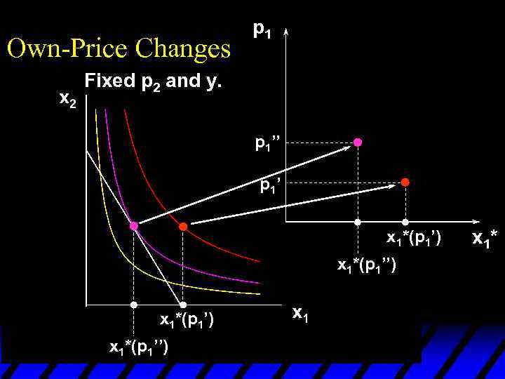
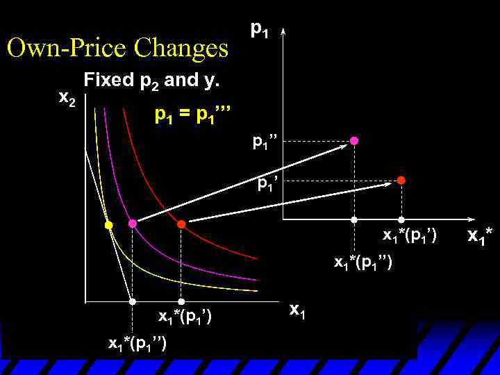
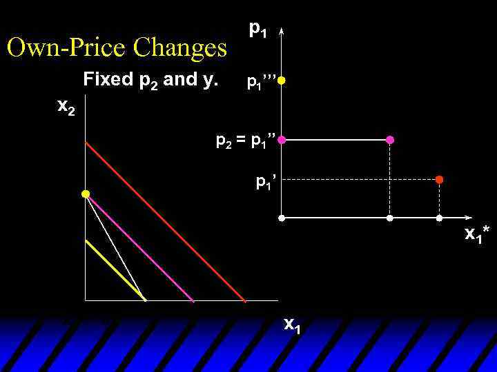
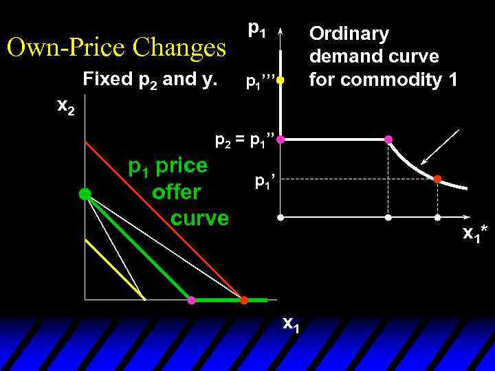
 Own-Price Changes u How does x 1*(p 1, p 2, y) change as p 1 changes, holding p 2 and y constant? u Suppose only p 1 increases, from p 1’ to p 1’’ and then to p 1’’’.
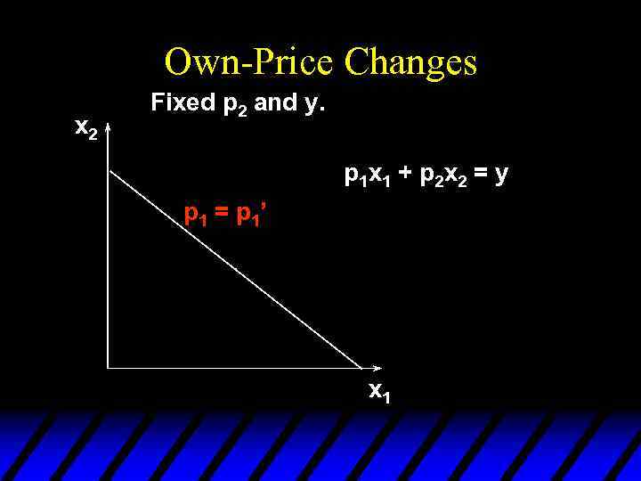 Own-Price Changes x 2 Fixed p 2 and y. p 1 x 1 + p 2 x 2 = y p 1 = p 1’ x 1
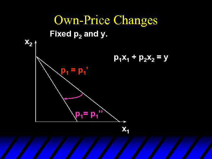 Own-Price Changes x 2 Fixed p 2 and y. p 1 x 1 + p 2 x 2 = y p 1 = p 1’ p 1= p 1’’ x 1
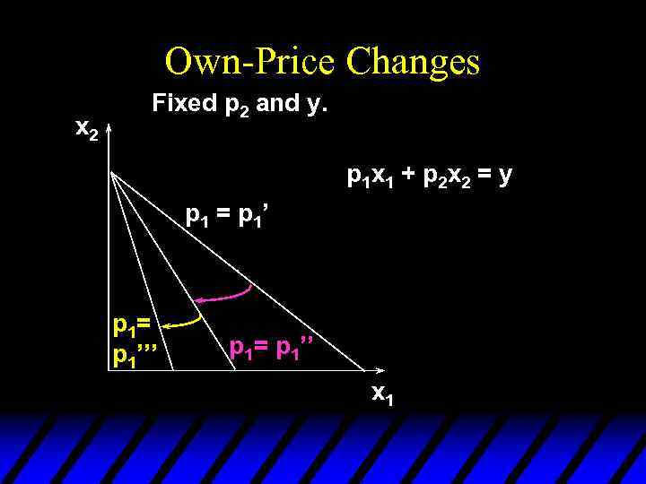 Own-Price Changes x 2 Fixed p 2 and y. p 1 x 1 + p 2 x 2 = y p 1 = p 1’ p 1= p 1’’ x 1
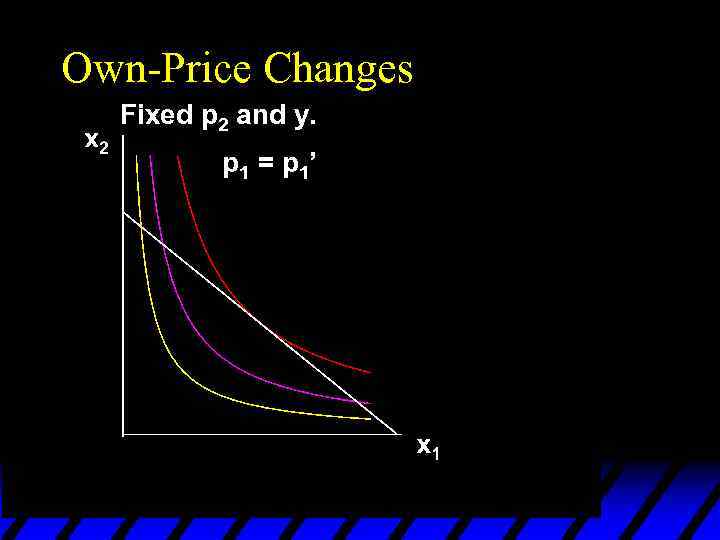 Own-Price Changes Fixed p 2 and y. p 1 = p 1’
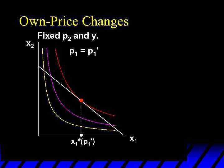 Own-Price Changes Fixed p 2 and y. p 1 = p 1’ x 1*(p 1’)
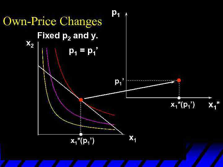 Own-Price Changes p 1 Fixed p 2 and y. p 1 = p 1’ x 1*(p 1’) x 1*
 Own-Price Changes p 1 Fixed p 2 and y. p 1 = p 1’’ p 1’ x 1*(p 1’) x 1*
 Own-Price Changes p 1 Fixed p 2 and y. p 1 = p 1’’ p 1’ x 1*(p 1’) x 1*(p 1’’) x 1*
 Own-Price Changes p 1 Fixed p 2 and y. p 1’’ p 1’ x 1*(p 1’) x 1*(p 1’’) x 1*
 Own-Price Changes p 1 Fixed p 2 and y. p 1 = p 1’’’ p 1’ x 1*(p 1’) x 1*(p 1’’) x 1*
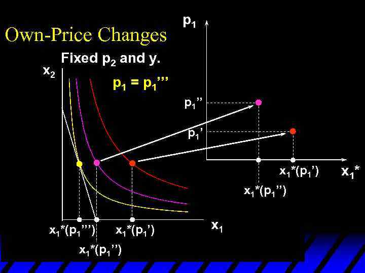 Own-Price Changes p 1 Fixed p 2 and y. p 1 = p 1’’’ p 1’ x 1*(p 1’) x 1*(p 1’’’) x 1*(p 1’’) x 1*
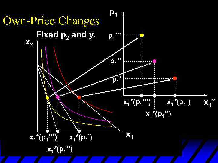 Own-Price Changes Fixed p 2 and y. p 1’’’ p 1’ x 1*(p 1’’’) x 1*(p 1’) x 1*(p 1’’) x 1*
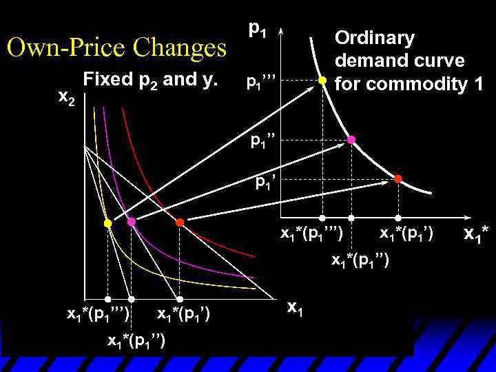 Own-Price Changes Fixed p 2 and y. p 1’’’ Ordinary demand curve for commodity 1 p 1’’ p 1’ x 1*(p 1’’’) x 1*(p 1’) x 1*(p 1’’) x 1*
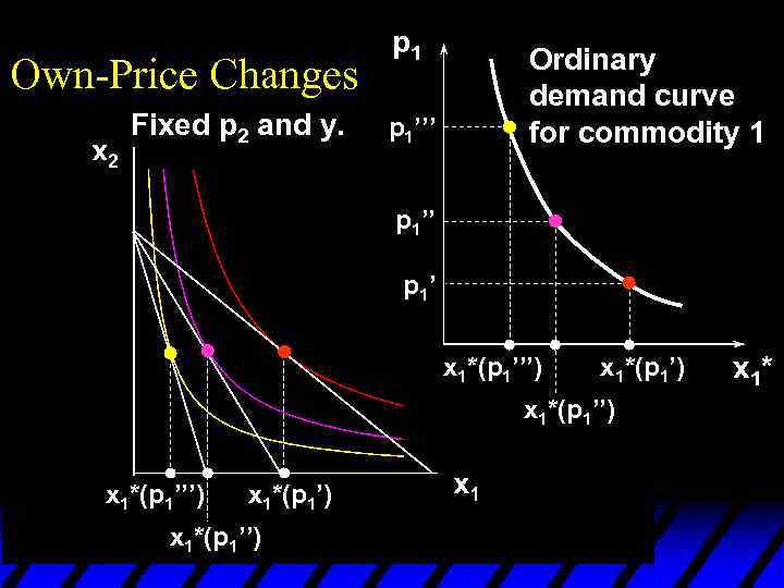 Own-Price Changes Fixed p 2 and y. p 1’’’ Ordinary demand curve for commodity 1 p 1’’ p 1’ x 1*(p 1’’’) x 1*(p 1’) x 1*(p 1’’) x 1*
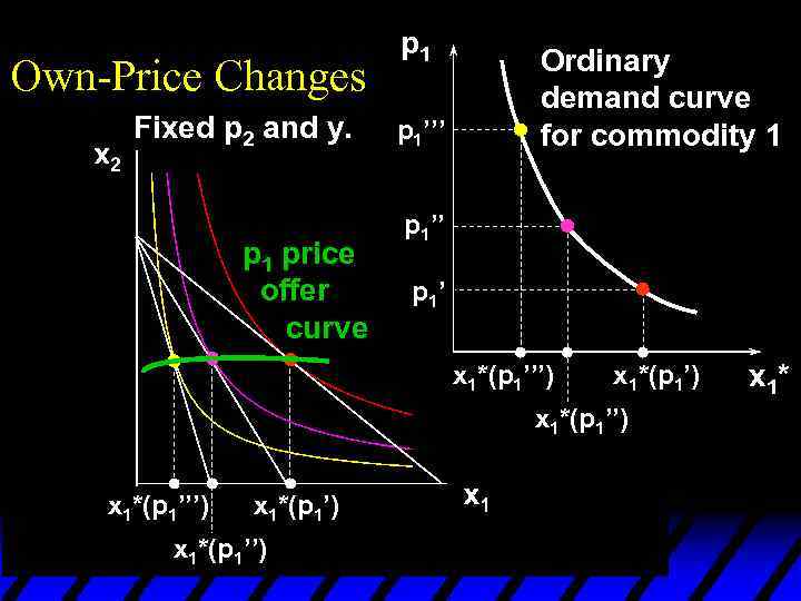 Own-Price Changes Fixed p 2 and y. p 1 price offer curve p 1’’’ Ordinary demand curve for commodity 1 p 1’’ p 1’ x 1*(p 1’’’) x 1*(p 1’) x 1*(p 1’’) x 1*
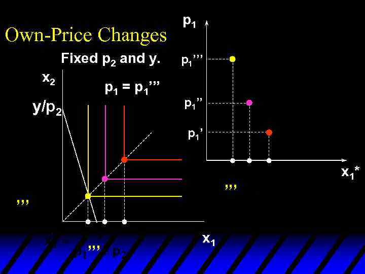
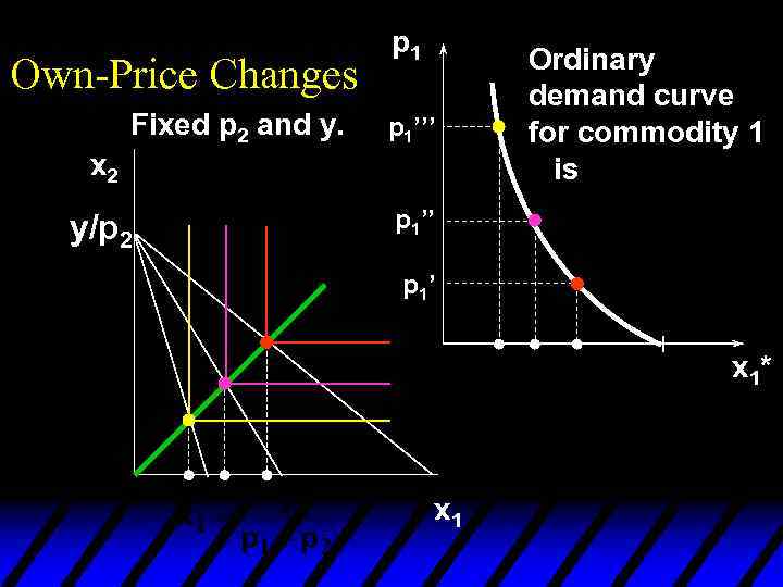
 Own-Price Changes u The curve containing all the utilitymaximizing bundles traced out as p 1 changes, with p 2 and y constant, is the p 1 - price offer curve. u The plot of the x 1 -coordinate of the p 1 - price offer curve against p 1 is the ordinary demand curve for commodity 1.
 Own-Price Changes u What does a p 1 price-offer curve look like for Cobb-Douglas preferences?
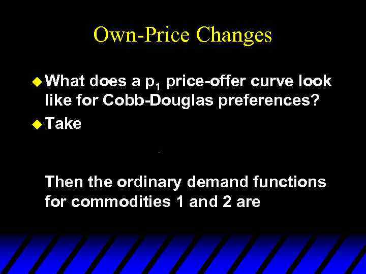 Own-Price Changes u What does a p 1 price-offer curve look like for Cobb-Douglas preferences? u Take Then the ordinary demand functions for commodities 1 and 2 are
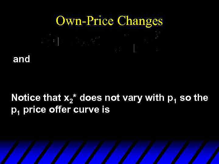 Own-Price Changes and Notice that x 2* does not vary with p 1 so the p 1 price offer curve is
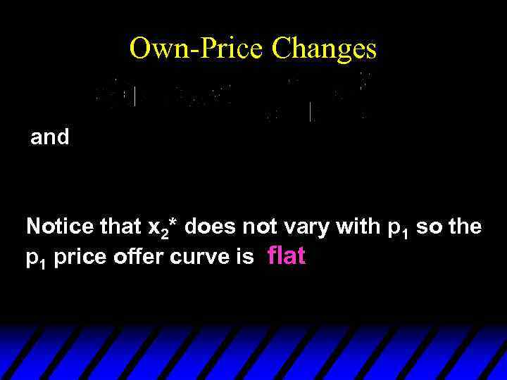 Own-Price Changes and Notice that x 2* does not vary with p 1 so the p 1 price offer curve is flat
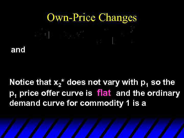 Own-Price Changes and Notice that x 2* does not vary with p 1 so the p 1 price offer curve is flat and the ordinary demand curve for commodity 1 is a
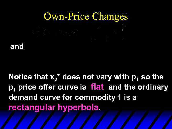 Own-Price Changes and Notice that x 2* does not vary with p 1 so the p 1 price offer curve is flat and the ordinary demand curve for commodity 1 is a rectangular hyperbola.
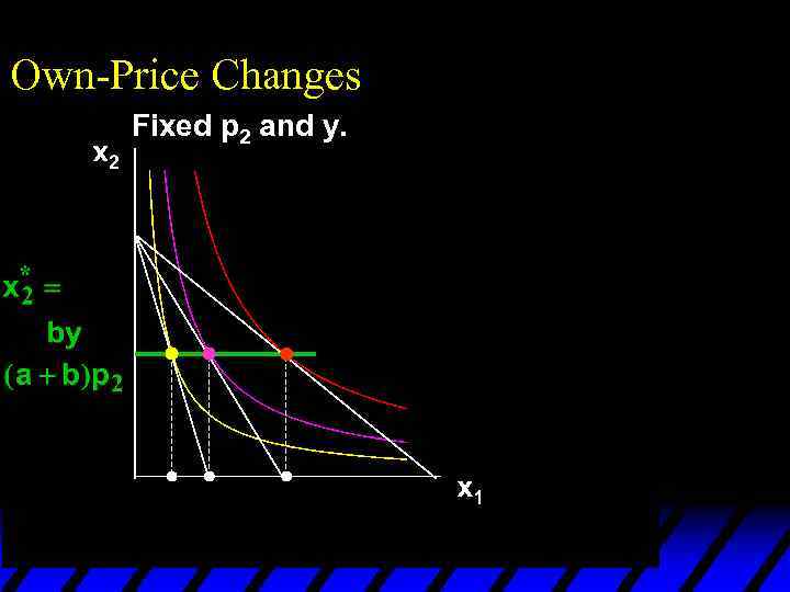 Own-Price Changes Fixed p 2 and y. x 1*(p 1’’’) x 1*(p 1’’)
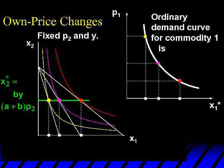 Own-Price Changes Fixed p 2 and y. p 1 Ordinary demand curve for commodity 1 is x 1*(p 1’’’) x 1*(p 1’’)
 Own-Price Changes u What does a p 1 price-offer curve look like for a perfect-complements utility function?
 Own-Price Changes u What does a p 1 price-offer curve look like for a perfect-complements utility function? Then the ordinary demand functions for commodities 1 and 2 are
 Own-Price Changes
 Own-Price Changes With p 2 and y fixed, higher p 1 causes smaller x 1* and x 2*.
 Own-Price Changes With p 2 and y fixed, higher p 1 causes smaller x 1* and x 2*. As
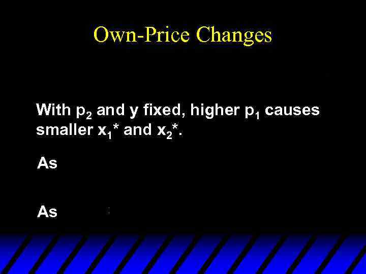 Own-Price Changes With p 2 and y fixed, higher p 1 causes smaller x 1* and x 2*. As As
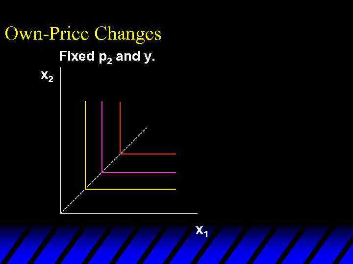 Own-Price Changes Fixed p 2 and y. x 2 x 1
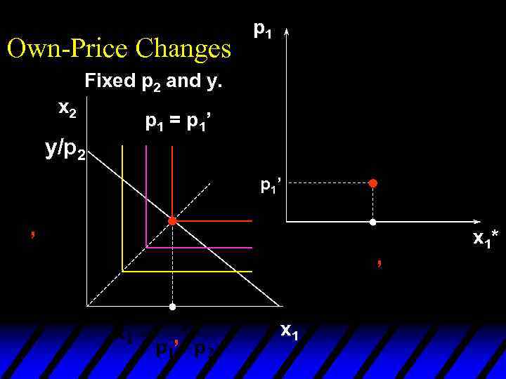 Own-Price Changes p 1 Fixed p 2 and y. x 2 y/p 2 p 1 = p 1’ x 1* ’ ’ ’ x 1
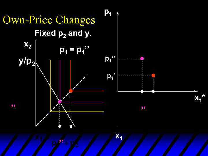 Own-Price Changes p 1 Fixed p 2 and y. x 2 y/p 2 p 1 = p 1’’ p 1’ x 1* ’’ ’’ ’’ x 1
 Own-Price Changes Fixed p 2 and y. x 2 p 1 = p 1’’’ y/p 2 p 1’’’ p 1’ ’’’ ’’’ x 1*
 Own-Price Changes Fixed p 2 and y. p 1’’’ x 2 y/p 2 Ordinary demand curve for commodity 1 is p 1’’ p 1’ x 1* x 1
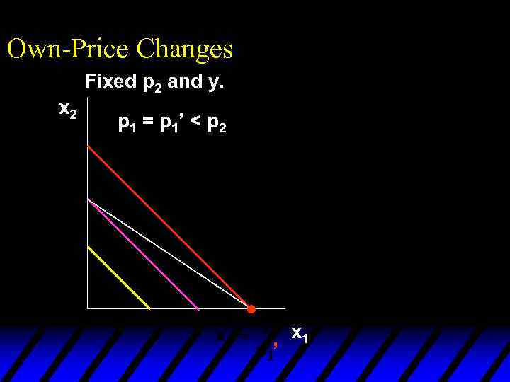
 Own-Price Changes u What does a p 1 price-offer curve look like for a perfect-substitutes utility function? Then the ordinary demand functions for commodities 1 and 2 are
 Own-Price Changes and
 Own-Price Changes Fixed p 2 and y. x 2 p 1 = p 1’ < p 2 ’ x 1
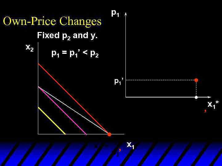 Own-Price Changes p 1 Fixed p 2 and y. x 2 p 1 = p 1’ < p 2 p 1’ ’ ’ x 1*
 Own-Price Changes p 1 Fixed p 2 and y. x 2 p 1 = p 1’’ = p 2 p 1’ x 1* x 1
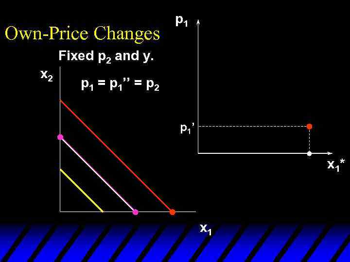 Own-Price Changes p 1 Fixed p 2 and y. x 2 p 1 = p 1’’ = p 2 p 1’ x 1* x 1
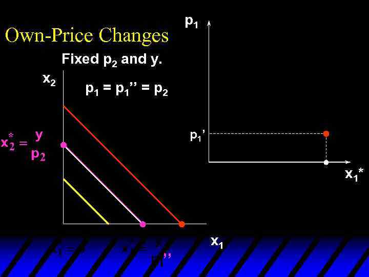 Own-Price Changes p 1 Fixed p 2 and y. x 2 p 1 = p 1’’ = p 2 p 1’ x 1* ’’ x 1
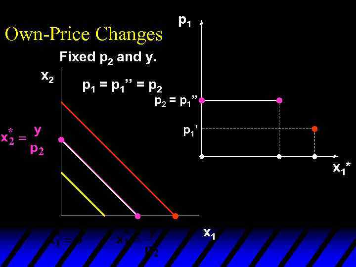 Own-Price Changes p 1 Fixed p 2 and y. x 2 p 1 = p 1’’ = p 2 = p 1’’ p 1’ x 1* x 1
 Own-Price Changes Fixed p 2 and y. p 1’’’ x 2 p 2 = p 1’’ p 1’ x 1* x 1
 Own-Price Changes Fixed p 2 and y. p 1 Ordinary demand curve for commodity 1 p 1’’’ x 2 p 2 = p 1’’ p 1 price offer curve p 1’ x 1* x 1
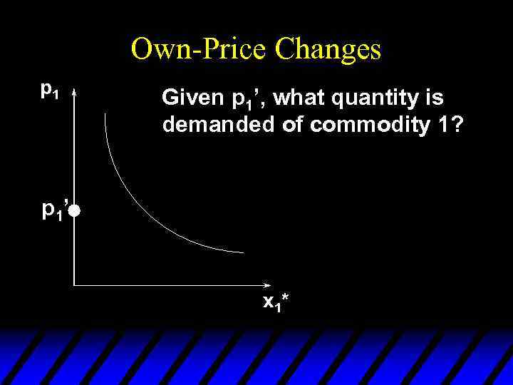
 Own-Price Changes u Usually we ask “Given the price for commodity 1 what is the quantity demanded of commodity 1? ” u But we could also ask the inverse question “At what price for commodity 1 would a given quantity of commodity 1 be demanded? ”
 Own-Price Changes p 1 Given p 1’, what quantity is demanded of commodity 1? p 1’ x 1*
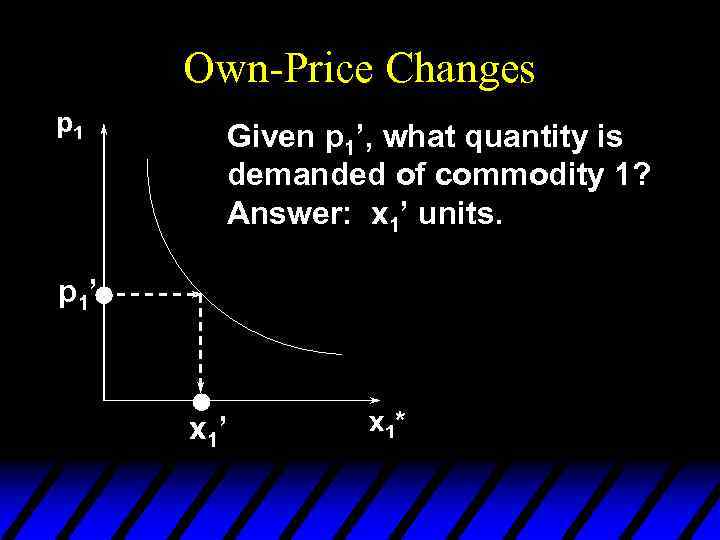 Own-Price Changes p 1 Given p 1’, what quantity is demanded of commodity 1? Answer: x 1’ units. p 1’ x 1*
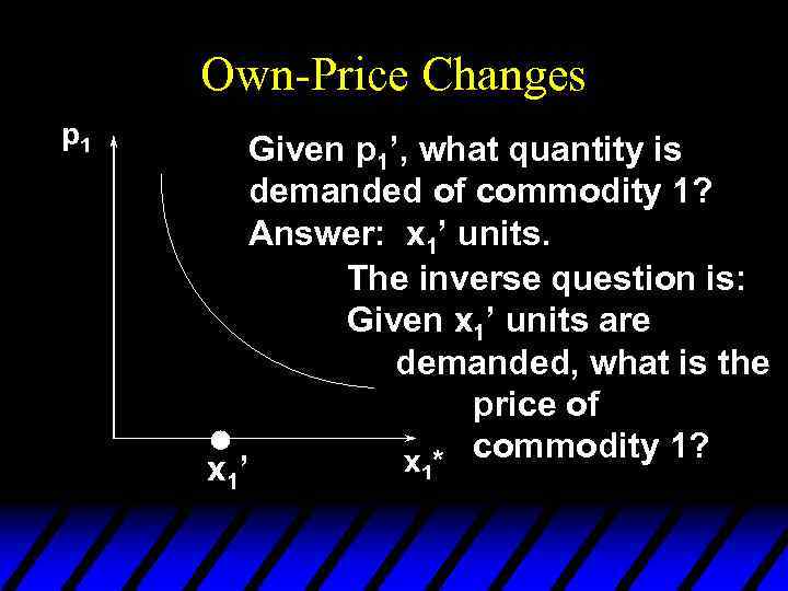 Own-Price Changes p 1 Given p 1’, what quantity is demanded of commodity 1? Answer: x 1’ units. The inverse question is: Given x 1’ units are demanded, what is the price of x 1* commodity 1? x 1’
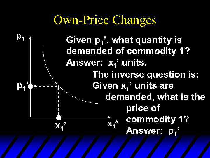 Own-Price Changes p 1’ Given p 1’, what quantity is demanded of commodity 1? Answer: x 1’ units. The inverse question is: Given x 1’ units are demanded, what is the price of x 1* commodity 1? x 1’ Answer: p 1’
 Own-Price Changes u Taking quantity demanded as given and then asking what must be price describes the inverse demand function of a commodity.
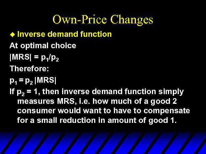 Own-Price Changes u Inverse demand function At optimal choice |MRS| = p 1/p 2 Therefore: p 1 = p 2 |MRS| If p 2 = 1, then inverse demand function simply measures MRS, i. e. how much of a good 2 consumer would want to have to compensate for a small reduction in amount of good 1.
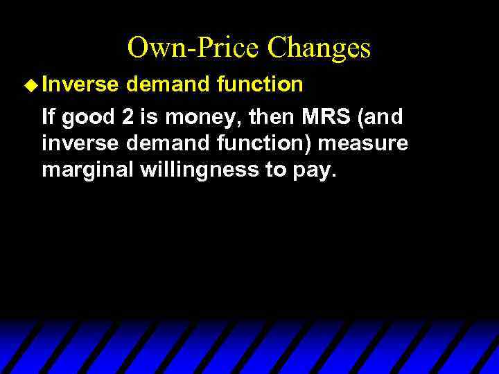 Own-Price Changes u Inverse demand function If good 2 is money, then MRS (and inverse demand function) measure marginal willingness to pay.
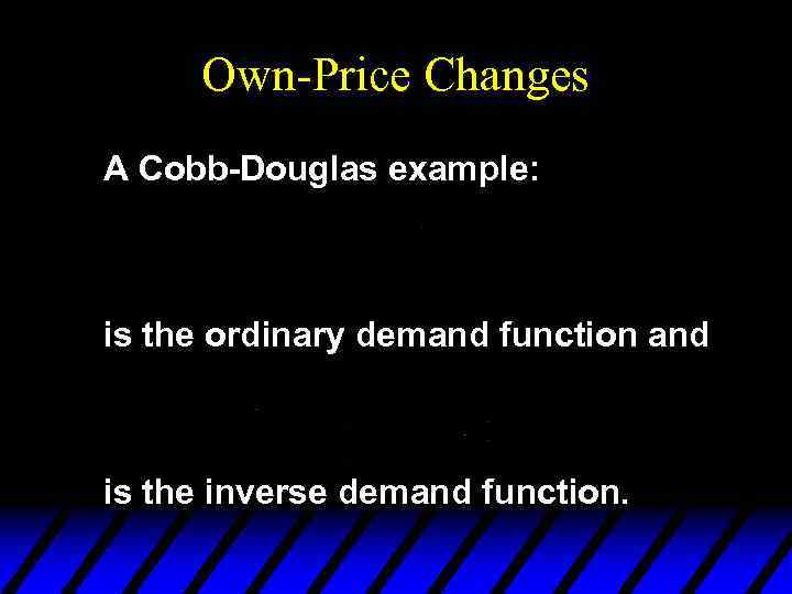 Own-Price Changes A Cobb-Douglas example: is the ordinary demand function and is the inverse demand function.
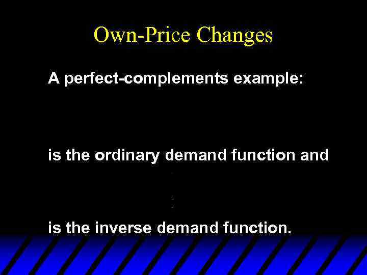 Own-Price Changes A perfect-complements example: is the ordinary demand function and is the inverse demand function.
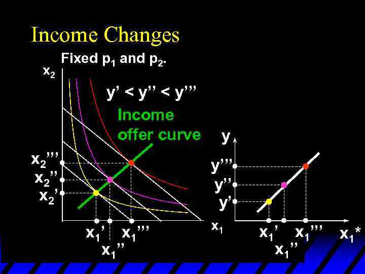
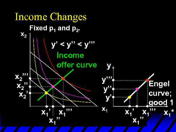
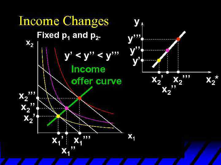
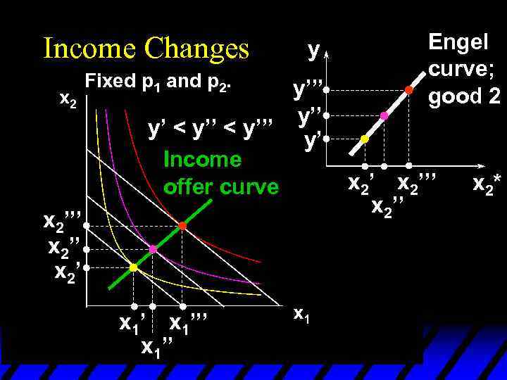
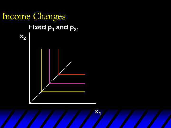
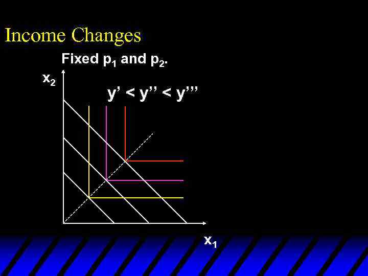
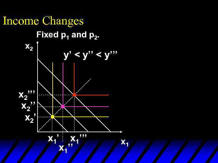
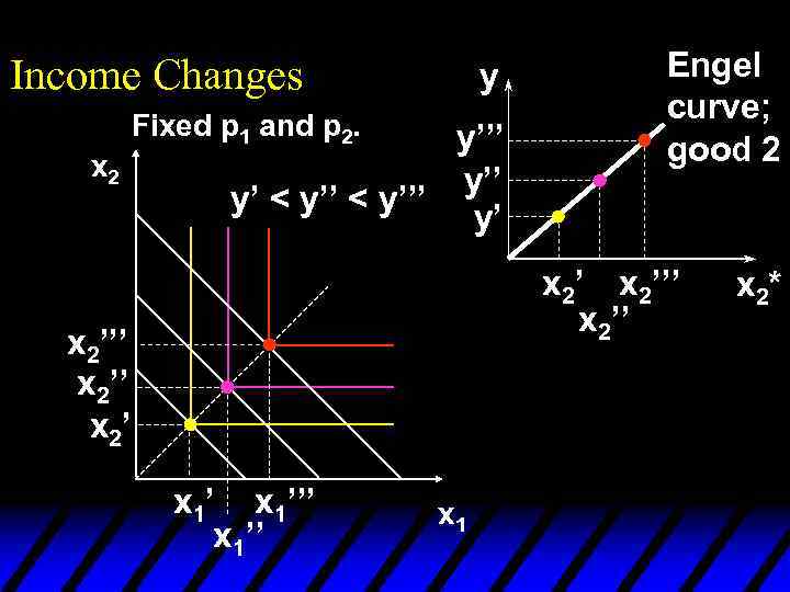
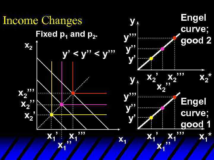
 Income Changes u How does the value of x 1*(p 1, p 2, y) change as y changes, holding both p 1 and p 2 constant?
 Income Changes Fixed p 1 and p 2. y’ < y’’’
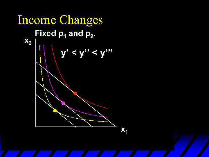 Income Changes Fixed p 1 and p 2. y’ < y’’’
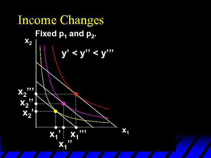 Income Changes Fixed p 1 and p 2. y’ < y’’’ x 2’’ x 2’ x 1’’’ x 1’’
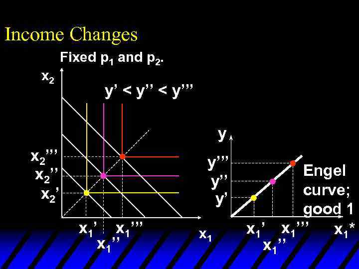
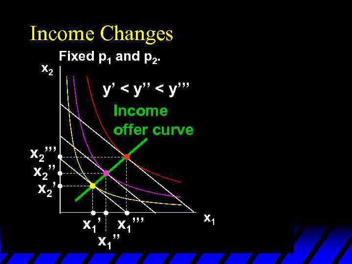 Income Changes Fixed p 1 and p 2. y’ < y’’’ Income offer curve x 2’’’ x 2’ x 1’’’ x 1’’
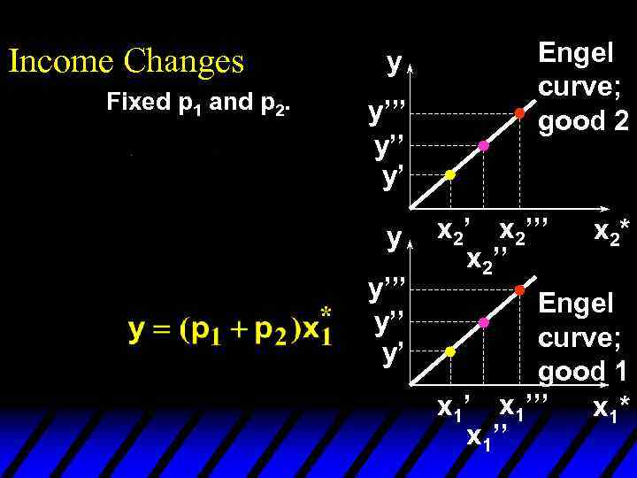
 Income Changes u. A plot of quantity demanded against income is called an Engel curve.
 Income Changes Fixed p 1 and p 2. y’ < y’’’ Income offer curve x 2’’’ x 2’ x 1’’’ x 1’’
 Income Changes Fixed p 1 and p 2. y’ < y’’’ Income offer curve x 2’’’ x 2’ y y’’’ y’ x 1’’’ x 1’’’ x 1* x 1’’
 Income Changes Fixed p 1 and p 2. y’ < y’’’ Income offer curve x 2’’’ x 2’ y y’’’ y’ x 1’’’ x 1’’ Engel curve; good 1 x 1’’’ x 1* x 1’’
 Income Changes y Fixed p 1 and p 2. y’’’ y’ < y’’’ y’ Income offer curve x 2’’’ x 2’ x 1’’’ x 1’’ x 2’’’ x 2*
 Income Changes Fixed p 1 and p 2. y y’’’ y’ < y’’’ y’ Income offer curve x 2’’’ x 2’ x 1’’’ x 1’’ Engel curve; good 2 x 2’’’ x 2*
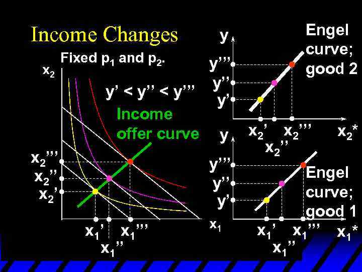 Income Changes y Fixed p 1 and p 2. y’’’ y’ < y’’’ y’ Income offer curve y x 2’’’ x 2’ y’’ y’ x 1’’’ x 1’’ Engel curve; good 2 x 2’’’ x 2* Engel curve; good 1 x 1’’’ x 1* x 1’’
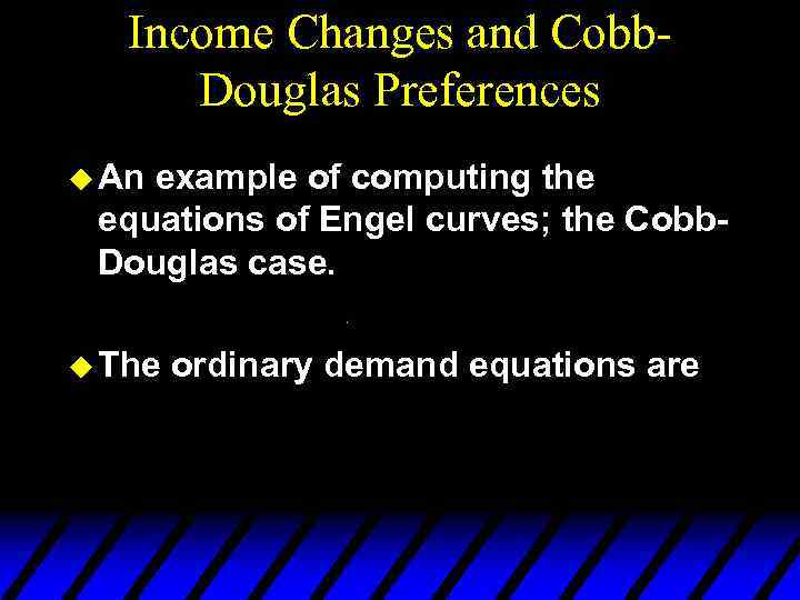 Income Changes and Cobb. Douglas Preferences u An example of computing the equations of Engel curves; the Cobb. Douglas case. u The ordinary demand equations are
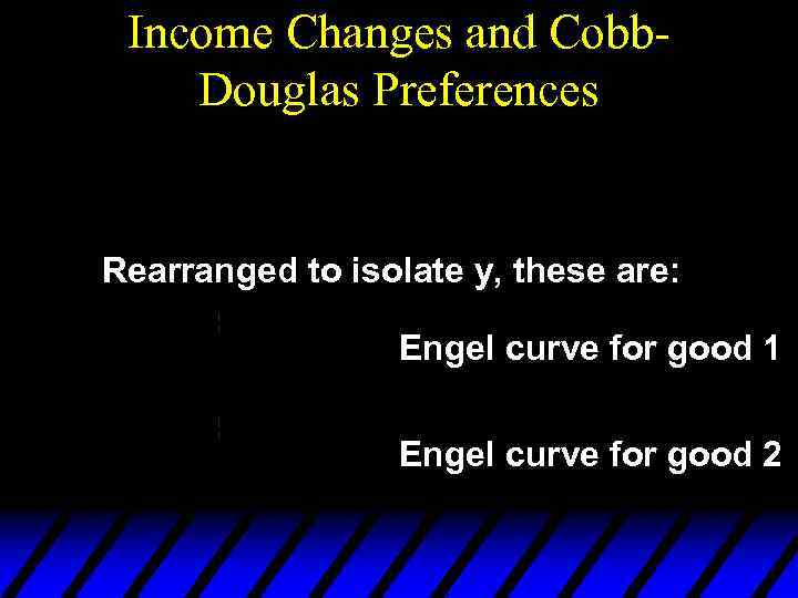 Income Changes and Cobb. Douglas Preferences Rearranged to isolate y, these are: Engel curve for good 1 Engel curve for good 2
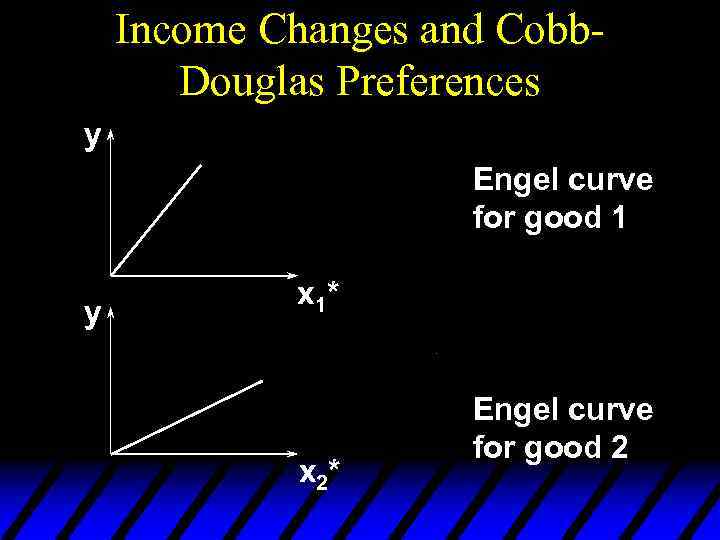 Income Changes and Cobb. Douglas Preferences y Engel curve for good 1 y x 1* x 2* Engel curve for good 2
 Income Changes and Perfectly. Complementary Preferences u Another example of computing the equations of Engel curves; the perfectly-complementary case. u The ordinary demand equations are
 Income Changes and Perfectly. Complementary Preferences Rearranged to isolate y, these are: Engel curve for good 1 Engel curve for good 2
 Income Changes Fixed p 1 and p 2. x 2 x 1
 Income Changes Fixed p 1 and p 2. x 2 y’ < y’’’ x 1
 Income Changes Fixed p 1 and p 2. x 2 y’ < y’’’ x 1
 Income Changes Fixed p 1 and p 2. x 2 y’ < y’’’ x 2’’ x 2’ x 1’’’ x 1
 Income Changes Fixed p 1 and p 2. x 2 y’ < y’’’ y x 2’’’ x 2’ y’’ y’ x 1’’’ x 1 Engel curve; good 1 x 1’’’ x 1* x 1’’
 Income Changes y Fixed p 1 and p 2. x 2 y’’’ y’ < y’’’ y’ Engel curve; good 2 x 2’’’ x 2’’ x 2’ x 1’’’ x 1 x 2*
 Income Changes y Fixed p 1 and p 2. x 2 y’’’ y’ < y’’’ y’ y x 2’’’ x 2’ y’’ y’ x 1’’’ x 1 Engel curve; good 2 x 2’’’ x 2* Engel curve; good 1 x 1’’’ x 1* x 1’’
 Income Changes Fixed p 1 and p 2. y y’’’ y’’ y’ Engel curve; good 2 x 2’’’ x 2* Engel curve; good 1 x 1’’’ x 1* x 1’’
 Income Changes and Perfectly. Substitutable Preferences u Another example of computing the equations of Engel curves; the perfectly-substitution case. u The ordinary demand equations are
 Income Changes and Perfectly. Substitutable Preferences
 Income Changes and Perfectly. Substitutable Preferences Suppose p 1 < p 2. Then
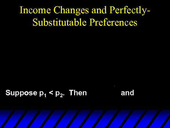 Income Changes and Perfectly. Substitutable Preferences Suppose p 1 < p 2. Then and
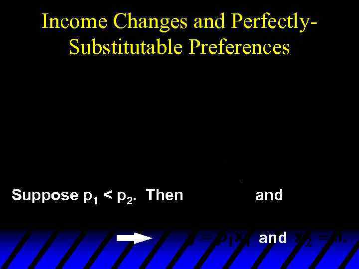 Income Changes and Perfectly. Substitutable Preferences Suppose p 1 < p 2. Then and
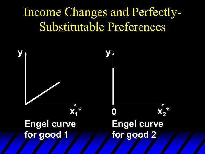 Income Changes and Perfectly. Substitutable Preferences y y x 1* Engel curve for good 1 x 2* 0 Engel curve for good 2
 Income Changes u In every example so far the Engel curves have all been straight lines? Q: Is this true in general? u A: No. Engel curves are straight lines if the consumer’s preferences are homothetic.
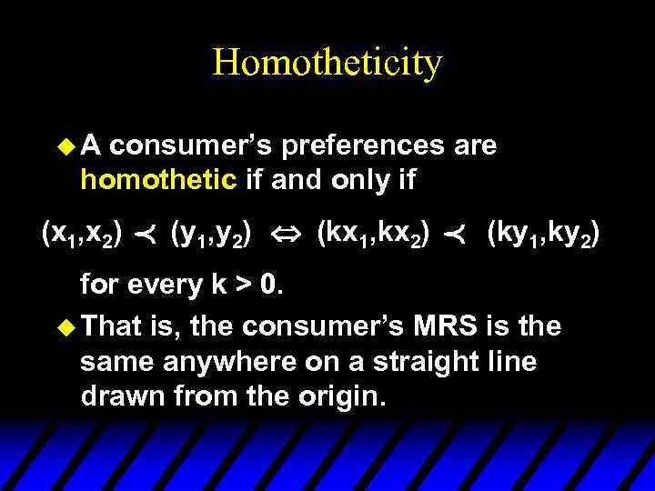 Homotheticity u. A consumer’s preferences are homothetic if and only if (x 1, x 2) p (y 1, y 2) Û (kx 1, kx 2) p (ky 1, ky 2) for every k > 0. u That is, the consumer’s MRS is the same anywhere on a straight line drawn from the origin.
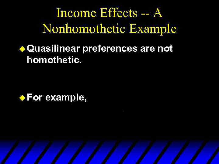 Income Effects -- A Nonhomothetic Example u Quasilinear preferences are not homothetic. u For example,
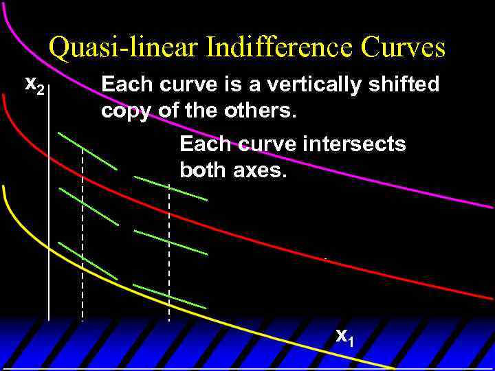 Quasi-linear Indifference Curves x 2 Each curve is a vertically shifted copy of the others. Each curve intersects both axes. x 1
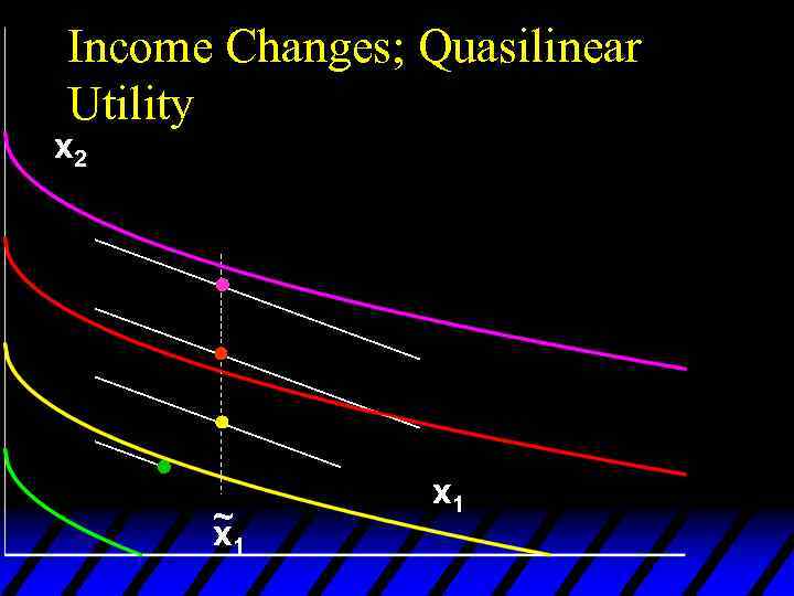 Income Changes; Quasilinear Utility x 2 ~ x 1
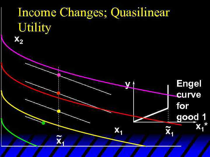 Income Changes; Quasilinear Utility x 2 y ~ x 1 Engel curve for good 1 x 1* ~ x 1
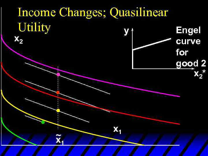 Income Changes; Quasilinear Utility y x 2 ~ x 1 Engel curve for good 2 x 2*
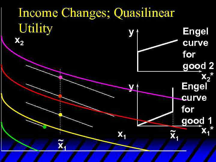 Income Changes; Quasilinear Utility y x 2 y ~ x 1 Engel curve for good 2 x 2* Engel curve for good 1 x 1* ~ x 1
 Income Effects u. A good for which quantity demanded rises with income is called normal. u Therefore a normal good’s Engel curve is positively sloped.
 Income Effects u. A good for which quantity demanded falls as income increases is called income inferior. u Therefore an income inferior good’s Engel curve is negatively sloped.
 Income Effects u In the US over last hundred years income increased many times whereas the number of kids per household went down. u Are children an inferior good?
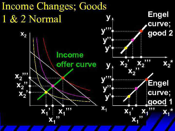 Income Changes; Goods y 1 & 2 Normal Income offer curve x 2’’’ x 2’ y’’ y’ y y’’’ y’ x 1’’’ x 1’’ Engel curve; good 2 x 2’’’ x 2* Engel curve; good 1 x 1’’’ x 1* x 1’’
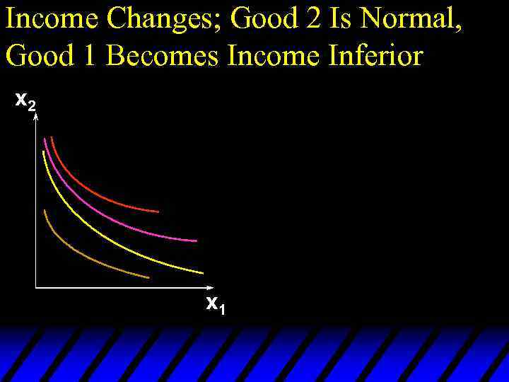 Income Changes; Good 2 Is Normal, Good 1 Becomes Income Inferior x 2 x 1
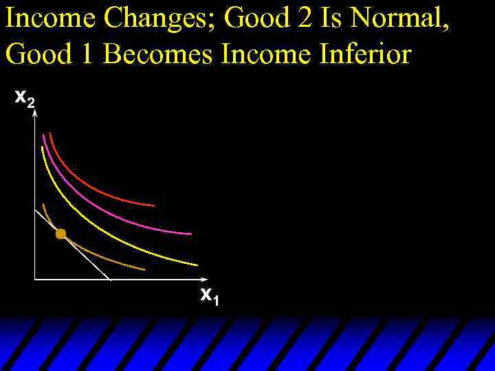 Income Changes; Good 2 Is Normal, Good 1 Becomes Income Inferior x 2 x 1
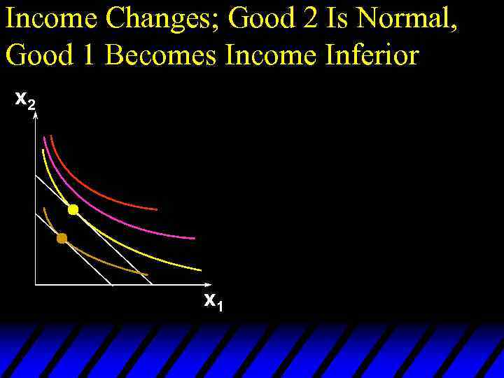 Income Changes; Good 2 Is Normal, Good 1 Becomes Income Inferior x 2 x 1
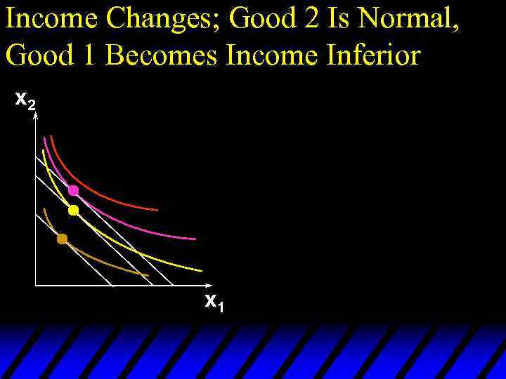 Income Changes; Good 2 Is Normal, Good 1 Becomes Income Inferior x 2 x 1
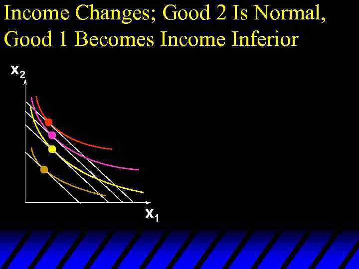 Income Changes; Good 2 Is Normal, Good 1 Becomes Income Inferior x 2 x 1
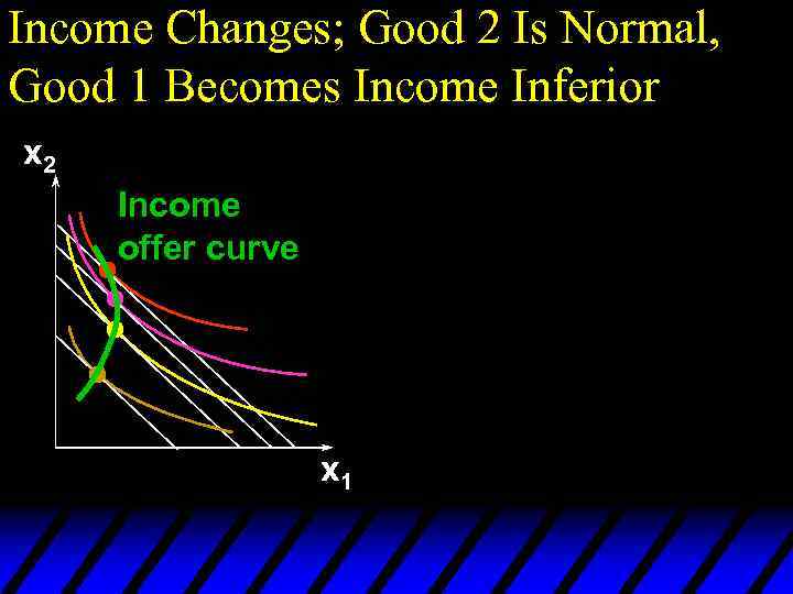 Income Changes; Good 2 Is Normal, Good 1 Becomes Income Inferior x 2 Income offer curve x 1
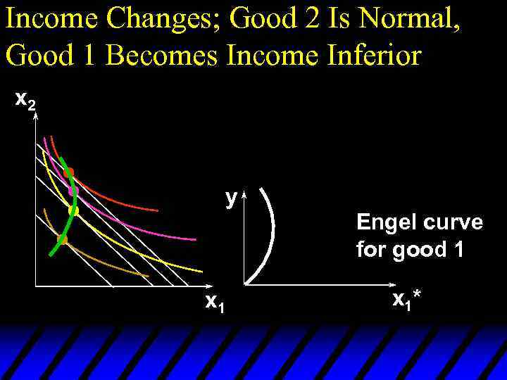 Income Changes; Good 2 Is Normal, Good 1 Becomes Income Inferior x 2 y Engel curve for good 1 x 1*
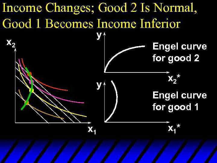 Income Changes; Good 2 Is Normal, Good 1 Becomes Income Inferior x 2 y Engel curve for good 2 y x 2* Engel curve for good 1 x 1*
 Ordinary Goods u. A good is called ordinary if the quantity demanded of it always increases as its own price decreases.
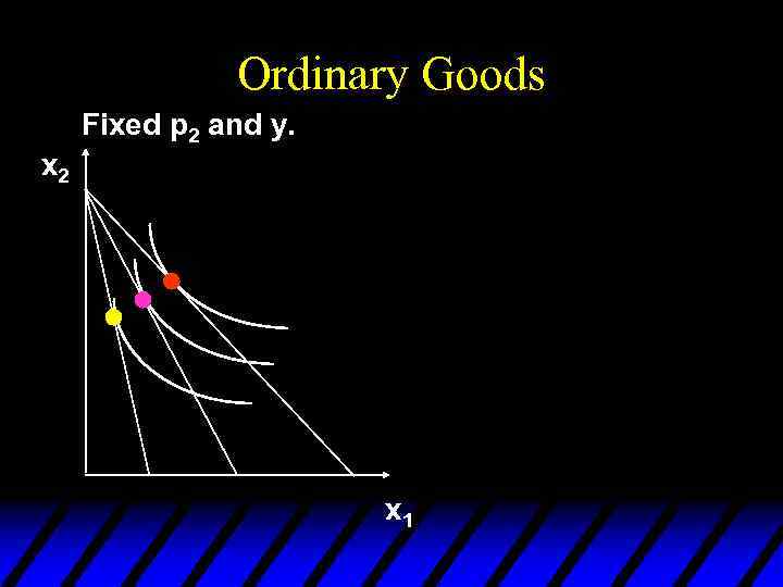 Ordinary Goods Fixed p 2 and y. x 2 x 1
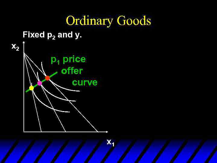 Ordinary Goods Fixed p 2 and y. x 2 p 1 price offer curve x 1
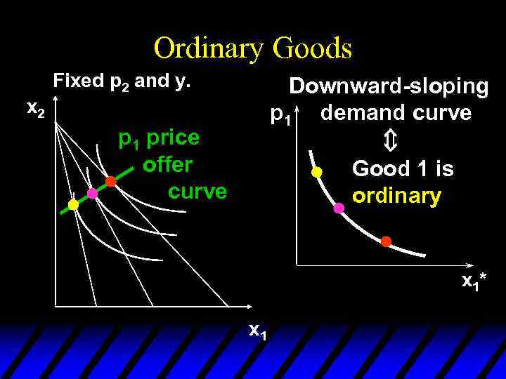 Ordinary Goods Fixed p 2 and y. Downward-sloping p 1 demand curve x 2 Û p 1 price offer curve Good 1 is ordinary x 1* x 1
 Giffen Goods u If, for some values of its own price, the quantity demanded of a good rises as its own-price increases then the good is called Giffen.
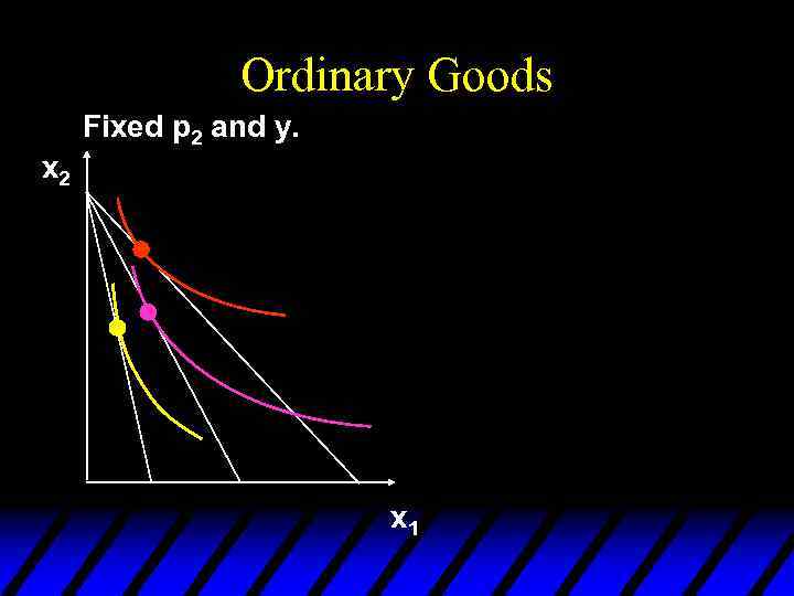 Ordinary Goods Fixed p 2 and y. x 2 x 1
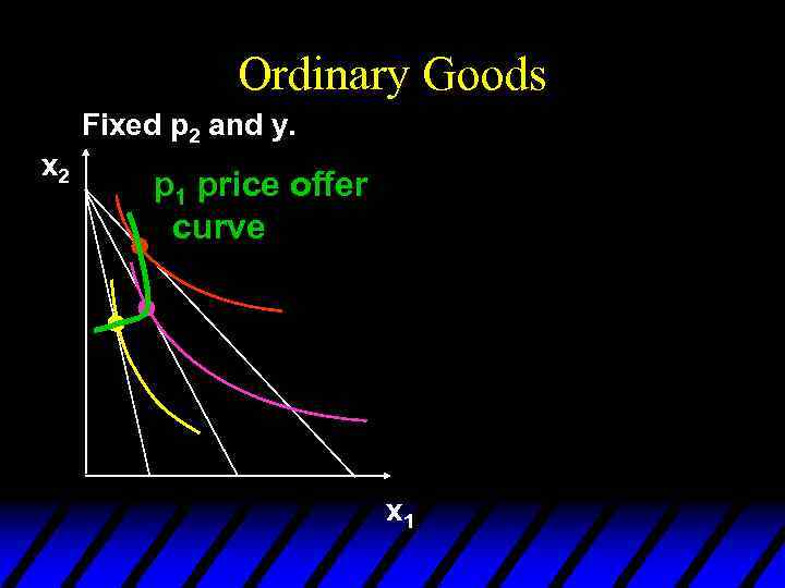 Ordinary Goods Fixed p 2 and y. x 2 p 1 price offer curve x 1
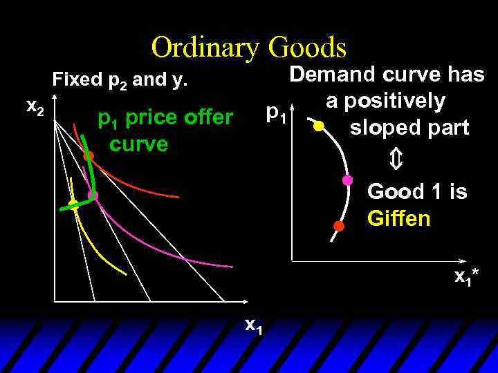 Ordinary Goods Demand curve has a positively p 1 sloped part Fixed p 2 and y. x 2 Û p 1 price offer curve Good 1 is Giffen x 1* x 1
 Cross-Price Effects u If an increase in p 2 – increases demand for commodity 1 then commodity 1 is a gross substitute for commodity 2. – reduces demand for commodity 1 then commodity 1 is a gross complement for commodity 2.
 Cross-Price Effects A perfect-complements example: so Therefore commodity 2 is a gross complement for commodity 1.
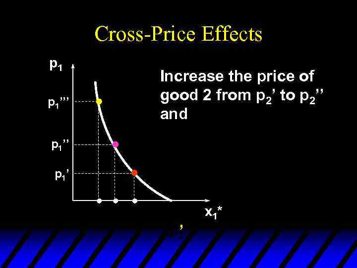 Cross-Price Effects p 1’’’ Increase the price of good 2 from p 2’ to p 2’’ and p 1’’ p 1’ x 1* ’
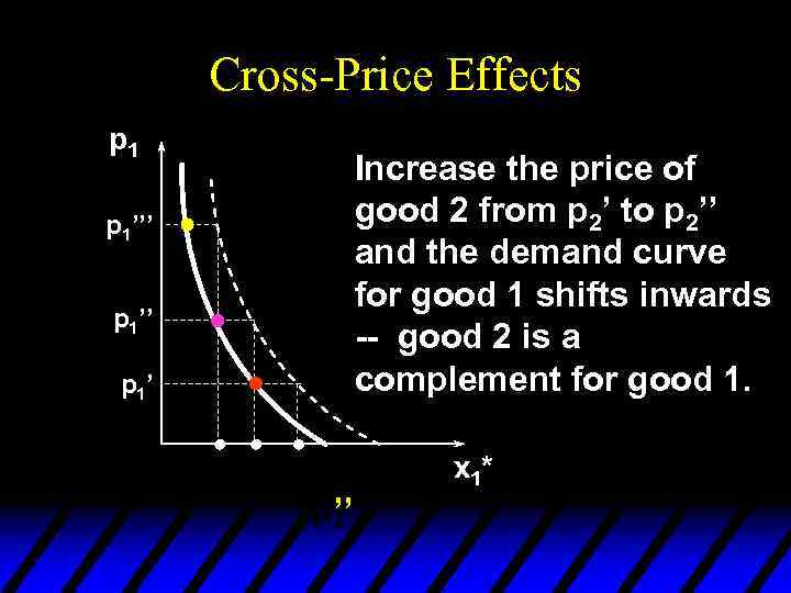 Cross-Price Effects p 1 Increase the price of good 2 from p 2’ to p 2’’ and the demand curve for good 1 shifts inwards -- good 2 is a complement for good 1. p 1’’’ p 1’ x 1* ’’
 Cross-Price Effects A Cobb- Douglas example: so
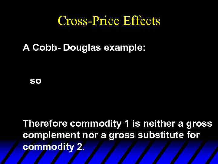 Cross-Price Effects A Cobb- Douglas example: so Therefore commodity 1 is neither a gross complement nor a gross substitute for commodity 2.


