Chapter Seven Costs 2008 Pearson Addison Wesley

Chapter Seven Costs © 2008 Pearson Addison Wesley. All rights reserved

無人商店紅什麼？小白店員絕跡 (中央社訊息服務 20091127 16: 13) • 近年來消費者自主意識抬頭，自助旅行、自助加油站、自 助租片店、自助洗衣店等消費習慣走紅，也讓新一代智慧 型無人商店領導品牌「Mini. Shop 24 H無人商店」趁勢崛起， 還意外成為上班族兼差首選。。 • 創立「Mini. Shop 24 H無人商店」的優活力企業董座縱曜光說， 一般認為「無人商店」最大的優勢，在於零人事、庫存成 本，並能真正做到以「最小成本創造最大獲利」的營運績 效，但Mini. Shop更要做到用最方便、輕鬆的方式，滿足消費 者最深層的渴望。 資料來源：http: //tw. news. yahoo. com/article/url/d/a/091127/5/1 vsua. html (Mini Shop)

擴大台廠代 為日數位相機廠逆境求生活路 (中央社記者韓婷婷台北 15日電) • 金融風暴及日圓強勁升值重擊，「低價、超值」成為數位 相機市場新顯學，台灣代 廠商擁有設計、成本及快速應 變能力優勢，成為日本數位相機廠逆境求生少不了的夥伴 • 日廠為了避免市佔率流失，並且縮減資本支出，紛紛擴大 委外代 比率，以降低成本，尋求利潤最大化。原本一度 傳出退出市場的Fujifilm就是一個鮮明的例子。去年 12月下 旬，剛就任Fujifilm電子影像事業部長的 ( 木通)口武常務執 行董事為徹底改革成本構造，要求「從原料採購到生產完 成的前置作業時間要縮短一半，並降低製造成本 20%」。

擴大台廠代 為日數位相機廠逆境求生活路 (中央社記者韓婷婷台北 15日電) • 富士找來台灣最大代 廠華晶科順利完成，推出的Fujifilm A 170 數位相機，這款「俗又大碗」的殺手級產品，竟然成為富士逆 轉勝的關鍵球。日本專家認為，A 170能夠以低成本，還保留基 本應有功能，主要關鍵應該是「從產品設計到零件採購，大部 份都交給台灣的數位相機代 大廠一手包辦」 • 專家認為，後金融風暴時代，消費行為有了微妙的變化，「品 牌優先」觀念逐漸式微，起而代之的是「不管是誰，給我最好、 最便宜的」，只要誰能推出「便宜又超值」的產品，消費者就 買單。 資料來源：http: //tw. news. yahoo. com/article/url/d/a/091115/5/1 uzzi. html

Costs • In this chapter, we examine five main topics – Measuring Costs – Short-Run Costs – Long-Run Costs – Lower Costs in the Long Run – Cost of Producing Multiple Goods © 2008 Pearson Addison Wesley. All rights reserved. 7 -5

Economic Costs • Economic Cost – The economic cost or opportunity cost is the value of the best alternative use of a resource. © 2008 Pearson Addison Wesley. All rights reserved. 7 -6

Capital Costs • Two problems may arise in measuring the cost of capital. – The first is how to allocate the initial purchase cost over time. – The second is what to do if the value of the capital changes over time. • Durable Good – a product that is usable for years © 2008 Pearson Addison Wesley. All rights reserved. 7 -7

Allocating Capital Costs over Time • An economist amortizes the cost of the truck on the basis of its opportunity cost at each moment of time, which is the amount that the firm could charge others to rent the truck. © 2008 Pearson Addison Wesley. All rights reserved. 7 -8

Actual and Historical Costs • A piece of capital may be worth much more or much less today than it was when it was purchased. • The firm’s current opportunity cost of capital may be less than what it paid if the firm cannot resell the capital. • Sunk Cost – an expenditure that cannot be recovered © 2008 Pearson Addison Wesley. All rights reserved. 7 -9

Short-Run Costs • Short-Run Cost Measures 1) fixed cost (F) – a production expense that does not vary with output 2) variable cost (VC) – a production expense that changes with the quantity of output produced 3) cost (total cost, C) – the sum of a firm’s variable cost and fixed cost: C = VC + F © 2008 Pearson Addison Wesley. All rights reserved. 7 -10

Marginal Cost • A firm’s marginal cost (MC) is the amount by which a firm’s cost changes if the firm produces one more unit of output. • The marginal cost is: (7. 1) © 2008 Pearson Addison Wesley. All rights reserved. 7 -11

Average Costs • average fixed cost (AFC) – the fixed cost divided by the units of output produced: AFC = F/q • average variable cost (AVC) – the variable cost divided by the units of output produced: AVC = VC/q © 2008 Pearson Addison Wesley. All rights reserved. 7 -12

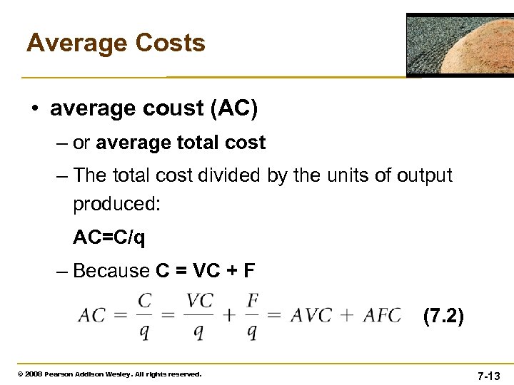Average Costs • average coust (AC) – or average total cost – The total cost divided by the units of output produced: AC=C/q – Because C = VC + F (7. 2) © 2008 Pearson Addison Wesley. All rights reserved. 7 -13

Short-Run Cost Curves • The total cost differs from the variable cost by the fixed cost. • The marginal cost curve, MC, cuts the average variable cost, AVC, and average cost, AC, curves at their minimums. © 2008 Pearson Addison Wesley. All rights reserved. 7 -14

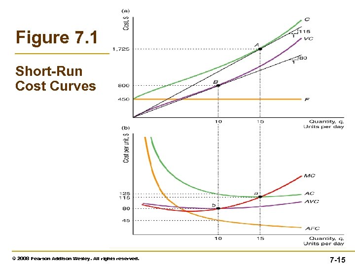Figure 7. 1 Short-Run Cost Curves © 2008 Pearson Addison Wesley. All rights reserved. 7 -15

Production Functions and the Shape of Cost Curves • The production function determines the shape of a firm’s cost curves. • The production function shows the amount of inputs needed to produce a given level of output. © 2008 Pearson Addison Wesley. All rights reserved. 7 -16

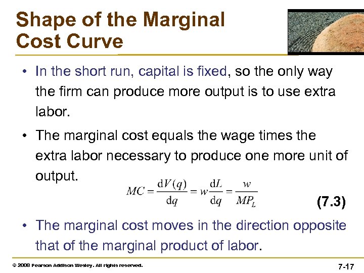Shape of the Marginal Cost Curve • In the short run, capital is fixed, so the only way the firm can produce more output is to use extra labor. • The marginal cost equals the wage times the extra labor necessary to produce one more unit of output. (7. 3) • The marginal cost moves in the direction opposite that of the marginal product of labor. © 2008 Pearson Addison Wesley. All rights reserved. 7 -17

Shape of the Average Cost Curves • For the firm, whose only variable input is labor, variable cost is w. L, so average variable is: (7. 4) • With a constant wage, the average variable cost moves in the opposite direction of the average product of labor. • The average cost curve is the vertical sum of the average variable cost curve and the average fixed cost curve. © 2008 Pearson Addison Wesley. All rights reserved. 7 -18

Shape of the Average Cost Curves • If the average variable cost curve is U-shaped, adding the strictly falling average fixed cost makes the average cost fall more steeply than the average variable cost curve at low output levels. • At high output levels, the average cost and average variable cost curves differ by ever smaller amounts, as the average fixed cost, F/q, approaches zero. • The average cost curve is also U-shaped. © 2008 Pearson Addison Wesley. All rights reserved. 7 -19

Effects of Taxes on Costs • Taxes applied to a firm shift some or all of the marginal and average cost curves. • A specific tax affects the firm’s average cost, average variable cost, and marginal cost curves but not its average fixed cost curve. © 2008 Pearson Addison Wesley. All rights reserved. 7 -20

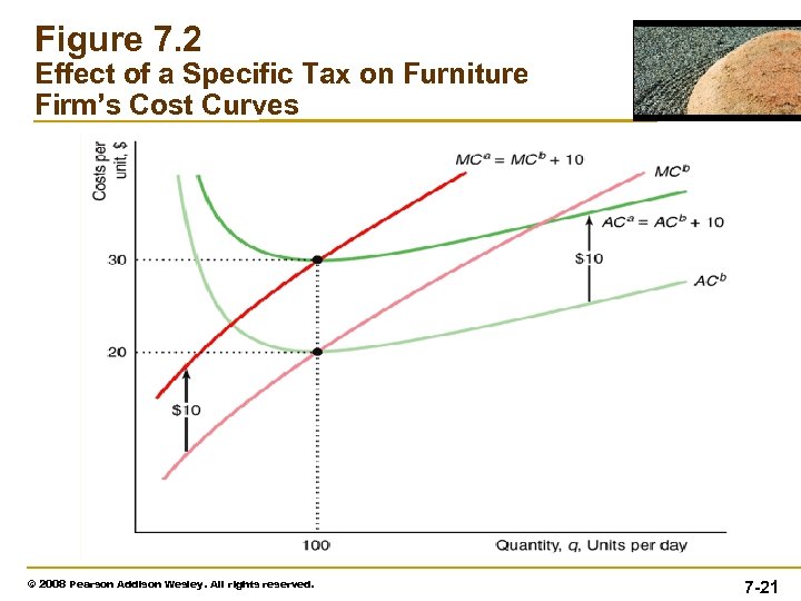Figure 7. 2 Effect of a Specific Tax on Furniture Firm’s Cost Curves © 2008 Pearson Addison Wesley. All rights reserved. 7 -21

Short-Run Cost Summary • In the short run, the cost associated with inputs that cannot be adjusted is fixed, while the cost from inputs that can be adjusted is variable. • Given constant input prices, the shapes of the cost, variable cost, marginal cost, and average cost curves are determined by the production function. © 2008 Pearson Addison Wesley. All rights reserved. 7 -22

Short-Run Cost Summary • Where there are diminishing marginal returns to a variable input, the variable cost and cost curves become relatively steep as output increases, so the average cost, average variable cost , and marginal cost curves rise with output. © 2008 Pearson Addison Wesley. All rights reserved. 7 -23

Short-Run Cost Summary • Both the average cost and average variable cost curve fall when marginal cost is below them and rise when marginal cost is above them, so the marginal cost curve cuts both of these average cost curves at their minimum points. © 2008 Pearson Addison Wesley. All rights reserved. 7 -24

Long-Run Costs • In the long run, the firm adjusts all its inputs so that its cost of production is as low as possible. • Although firms may incur fixed costs in the long run, these fixed costs are avoidable (rather than sunk, as in the short run). © 2008 Pearson Addison Wesley. All rights reserved. 7 -25

Input Choice • From among the technologically efficient combinations of inputs, a firm wants to choose the particular bundle with the lowest cost of production, which is the economically efficient combination of inputs. • To do so, the firm combines information about technology from the isoquant with information about the cost of labor and capital. © 2008 Pearson Addison Wesley. All rights reserved. 7 -26

Isocost Line • The firm’s total cost is the sum of its labor and capital cost (where r is the implicit rental rate): C = w. L + r. K (7. 6) • All the combinations of inputs that require the same (iso-) total expenditure (cost) (7. 7) • Using Algebra, (7. 8) © 2008 Pearson Addison Wesley. All rights reserved. 7 -27

Isocost Line • Three properties of isocost lines: – First, where the isocost lines hit the capital and labor axes depends on the firm’s cost and on the input prices. – Second, isocosts that are farther from the origin have higher costs than those that are closer to the origin. – Third, the slope of each isocost line is the same. © 2008 Pearson Addison Wesley. All rights reserved. 7 -28

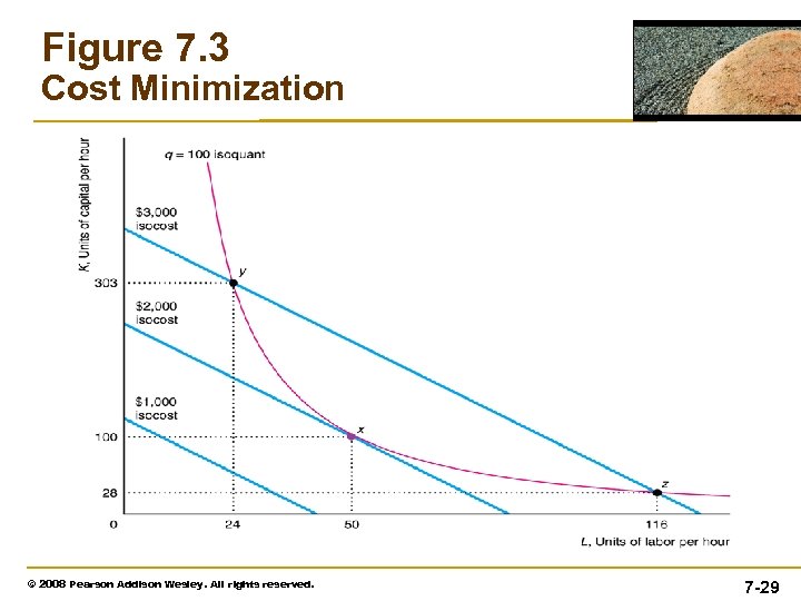Figure 7. 3 Cost Minimization © 2008 Pearson Addison Wesley. All rights reserved. 7 -29

Minimizing Cost • Lowest-isocost rule: – Pick the bundle of inputs where the lowest isocost line touches the isoquant. • Tangency rule: – Pick the bundle of inputs where the isoquant is tangent to the isocost line. • Last-dollar rule: – Pick the bundle of inputs where the last dollar spent on one input gives as much extra output as the last dollar spent on any other input. © 2008 Pearson Addison Wesley. All rights reserved. 7 -30

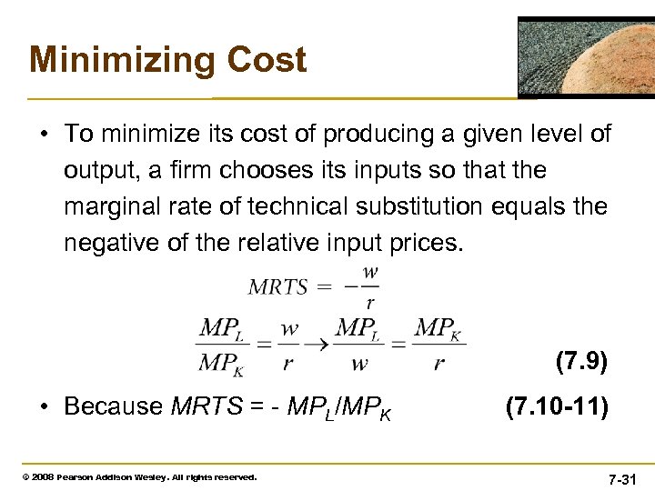Minimizing Cost • To minimize its cost of producing a given level of output, a firm chooses its inputs so that the marginal rate of technical substitution equals the negative of the relative input prices. (7. 9) • Because MRTS = - MPL/MPK © 2008 Pearson Addison Wesley. All rights reserved. (7. 10 -11) 7 -31

Using Calculus to Minimize Cost • Formally, the firm is minimizing its cost subject to the information in the production function contained in the isoquant expression. The corresponding Lagrangian problem is shown in Equation (7. 12). • Equation 7. 12 © 2008 Pearson Addison Wesley. All rights reserved. 7 -32

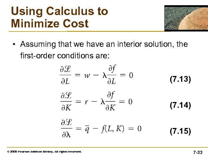Using Calculus to Minimize Cost • Assuming that we have an interior solution, the first-order conditions are: (7. 13) (7. 14) (7. 15) © 2008 Pearson Addison Wesley. All rights reserved. 7 -33

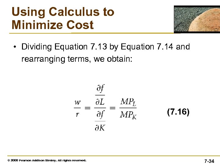Using Calculus to Minimize Cost • Dividing Equation 7. 13 by Equation 7. 14 and rearranging terms, we obtain: (7. 16) © 2008 Pearson Addison Wesley. All rights reserved. 7 -34

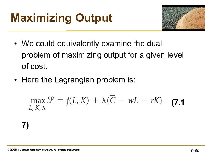Maximizing Output • We could equivalently examine the dual problem of maximizing output for a given level of cost. • Here the Lagrangian problem is: (7. 1 7) © 2008 Pearson Addison Wesley. All rights reserved. 7 -35

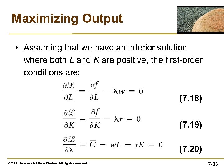Maximizing Output • Assuming that we have an interior solution where both L and K are positive, the first-order conditions are: (7. 18) (7. 19) (7. 20) © 2008 Pearson Addison Wesley. All rights reserved. 7 -36

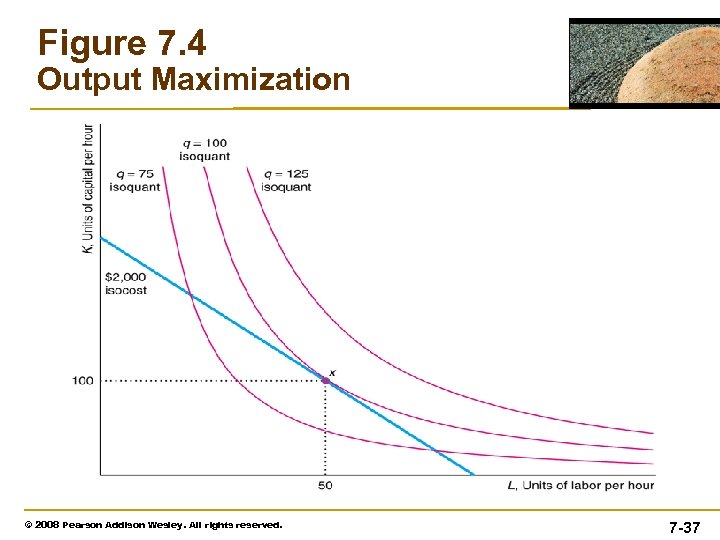Figure 7. 4 Output Maximization © 2008 Pearson Addison Wesley. All rights reserved. 7 -37

Factor Price Change • When the wage falls, the firm minimizes its new cost by substituting away from the now relatively more expensive input, capital, toward the now relatively less expensive input, labor. • The change in the wage does not affect technological efficiency, so it does not affect the isoquant. © 2008 Pearson Addison Wesley. All rights reserved. 7 -38

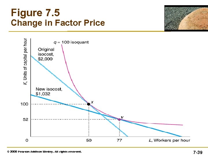Figure 7. 5 Change in Factor Price © 2008 Pearson Addison Wesley. All rights reserved. 7 -39

How Long-Run Cost Varies with Output • Expansion Path: – the cost-minimizing combination of labor and capital for each output level • Long-Run Cost Function – The expansion path contains the same information as its long-run cost function, C(q), which shown the relationship between the cost of production and output. © 2008 Pearson Addison Wesley. All rights reserved. 7 -40

Solved Problem 7. 4 • What is the expansion path function for a constant-return-to-scale Cobb-Douglas production function q = ALa. K 1 -a? • Use the tangency condition between the isocost and isoquant that determines the factor ratio when the firm is minimizing cost to derive the expansion path. (7. 21) © 2008 Pearson Addison Wesley. All rights reserved. 7 -41

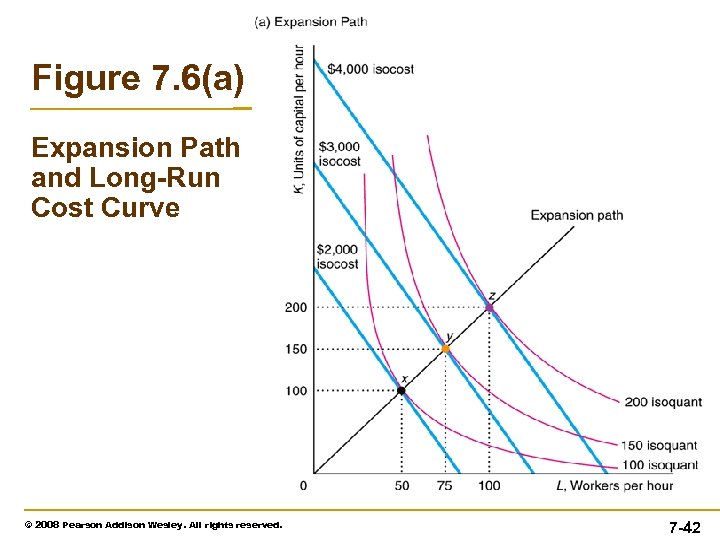Figure 7. 6(a) Expansion Path and Long-Run Cost Curve © 2008 Pearson Addison Wesley. All rights reserved. 7 -42

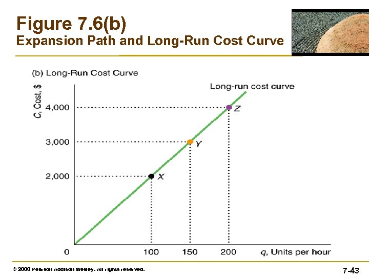Figure 7. 6(b) Expansion Path and Long-Run Cost Curve © 2008 Pearson Addison Wesley. All rights reserved. 7 -43

The Shape of Long-Run Cost Curves • The shapes of the average cost and marginal cost curves depend on the shape of the long-run cost curve. • As with the short-run curves, the shape of the long-run curves is determined by the production function relationship between output and inputs. • In the long run, returns to scale play a major role in determining the shape of the average cost curve and other cost curves. © 2008 Pearson Addison Wesley. All rights reserved. 7 -44

The Shape of Long-Run Cost Curves • Increasing all inputs in proportion may cause output to increase more than in proportion (increasing returns to scale) at low levels of output, in proportion (constant returns to scale) at intermediate levels of output, and less than in proportion (decreasing returns to scale) at high levels of output. • If a production function has this returns-to-scale pattern and the prices of inputs are constant, long-run average cost must be U-shaped. © 2008 Pearson Addison Wesley. All rights reserved. 7 -45

The Shape of Long-Run Cost Curves • Economies of Scale: – property of a cost function whereby the average cost of production falls as output expands • Diseconomies of Scale : – property of a cost function whereby the average cost of production rises when output increases © 2008 Pearson Addison Wesley. All rights reserved. 7 -46

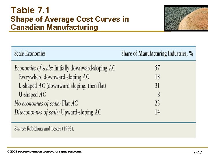Table 7. 1 Shape of Average Cost Curves in Canadian Manufacturing © 2008 Pearson Addison Wesley. All rights reserved. 7 -47

Lower Costs in the Long Run • Because the firm cannot vary its capital in the short run but vary it in the long run, short-run cost is at least as high as long-run cost and is higher if the “wrong” level of capital is used in the short run. • Long-Run Average Cost as the Envelope of Short-Run Average Cost Curves – As a result, the long-run average cost is always equal to or below the short-run average cost. © 2008 Pearson Addison Wesley. All rights reserved. 7 -48

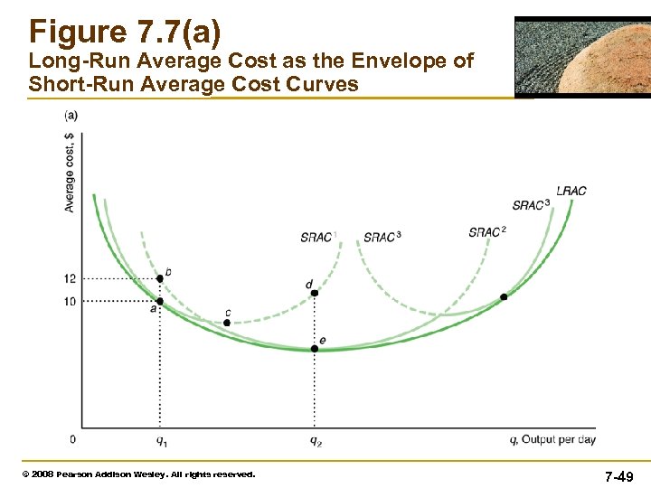Figure 7. 7(a) Long-Run Average Cost as the Envelope of Short-Run Average Cost Curves © 2008 Pearson Addison Wesley. All rights reserved. 7 -49

Figure 7. 7(b) Long-Run Average Cost as the Envelope of Short-Run Average Cost Curves © 2008 Pearson Addison Wesley. All rights reserved. 7 -50

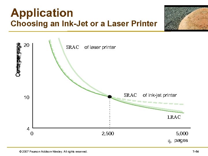
Application • 對台灣學生而言，在 2009年，採購家用印表機有噴墨式與黑白雷 射式兩種選擇。以印表機第一大廠hp為例，噴墨式印表機可選擇 hp deskjet D 1660，其單價為新台幣 990元，這款印表機黑白列印每 分鐘可達 20頁(黑白墨水匣平均可列印 200頁的標準頁面)，彩色列 印則每分鐘 16頁(黑白墨水匣平均可列印 165頁的標準頁面) ；而雷 射印表機如 hp Laser. Jet P 1006，黑白列印每分鐘可達 16頁，其單價 為新台幣 3, 888元 (碳粉匣平均可列印 1, 500 頁的標準頁面)。 資料來源： http: //buy. yahoo. com. tw/gdsale. asp? gdid=1751946 http: //buy. yahoo. com. tw/gdsale. asp? gdid=749845 http: //h 10060. www 1. hp. com/pageyield/index. html © 2008 Pearson Addison Wesley. All rights reserved. 7 -51

Application • Choosing an Ink-Jet or a Laser Printer: – You decide to buy a printer for your college assignments. You need to print in black and white. In 2007, you can buy a personal laser printer for $150 or an ink-jet printer for $75 that prints 15 pages a minute at 1, 200 dots per inch. © 2008 Pearson Addison Wesley. All rights reserved. 7 -52

Application • The cost of ink and paper is about 4 cents per page for a laser compared to about 7 cents per page for an ink jet. • The average cost per page of operating a laser is: $150/q + 0. 04 • The average cost per page of operating an ink jet: $75/q + 0. 07 © 2008 Pearson Addison Wesley. All rights reserved. 7 -53

Application Choosing an Ink-Jet or a Laser Printer 20 SRAC of laser printer SRAC 10 of ink-jet printer LRAC 4 0 © 2007 Pearson Addison-Wesley. All rights reserved. 2, 500 5, 000 q, pages 7– 54

Short-Run and Long-Run Expansion Paths • Long-run cost is lower than short-run cost because the firm has more flexibility in the long run. • To show the advantage of flexibility, we can compare the short-run and long-run expansion paths, which correspond to the short-run and long-run cost curves. © 2008 Pearson Addison Wesley. All rights reserved. 7 -55

Figure 7. 8 Long-Run and Short-Run Expansion Paths © 2008 Pearson Addison Wesley. All rights reserved. 7 -56

How Learning by Doing Lowers Costs • Learning by Doing : – the productive skills and knowledge of better ways to produce that workers and managers gain from experience. © 2008 Pearson Addison Wesley. All rights reserved. 7 -57

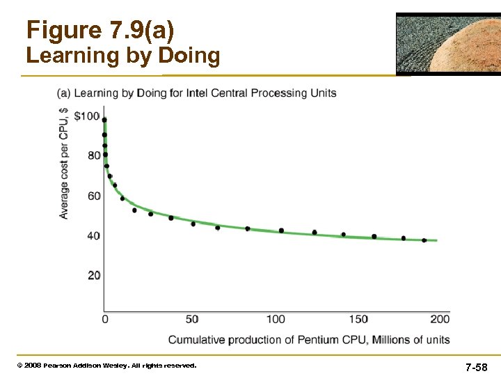Figure 7. 9(a) Learning by Doing © 2008 Pearson Addison Wesley. All rights reserved. 7 -58

Figure 7. 9(b) Learning by Doing © 2008 Pearson Addison Wesley. All rights reserved. 7 -59

Cost of Producing Multiple Goods • Few firms produce only a single good ─ We have discussed single-output firms only for simplicity. • If a firm produces two or more goods, the cost of one good may depend on the output level of the other. © 2008 Pearson Addison Wesley. All rights reserved. 7 -60

Cost of Producing Multiple Goods • We say that there are economies of scope if it is less expense to produce goods jointly than separately (Panzar and Willig, 1977, 1981). © 2008 Pearson Addison Wesley. All rights reserved. 7 -61

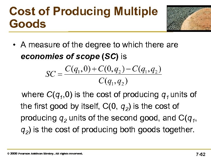Cost of Producing Multiple Goods • A measure of the degree to which there are economies of scope (SC) is where C(q 1, 0) is the cost of producing q 1 units of the first good by itself, C(0, q 2) is the cost of producing q 2 units of the second good, and C(q 1, q 2) is the cost of producing both goods together. © 2008 Pearson Addison Wesley. All rights reserved. 7 -62

Cost of Producing Multiple Goods • Production Possibility Frontier (PPF): – The maximum amount of outputs that can be produced from a fixed amount of input. – The production possibility frontier summarizes the trade-off someone faces. © 2008 Pearson Addison Wesley. All rights reserved. 7 -63

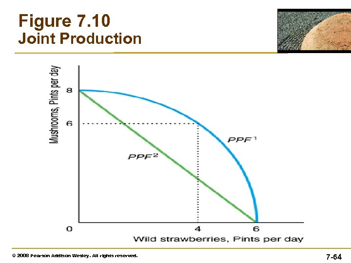Figure 7. 10 Joint Production © 2008 Pearson Addison Wesley. All rights reserved. 7 -64