Chapter Five Consumer Welfare and Policy Analysis

Chapter Five Consumer Welfare and Policy Analysis © 2008 Pearson Addison Wesley. All rights reserved

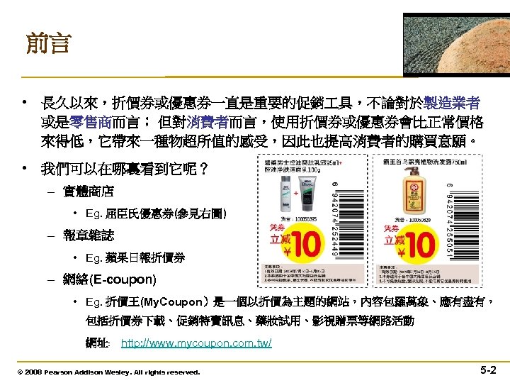前言 • 長久以來，折價券或優惠券一直是重要的促銷 具，不論對於製造業者 或是零售商而言； 但對消費者而言，使用折價券或優惠券會比正常價格 來得低，它帶來一種物超所值的感受，因此也提高消費者的購買意願。 • 我們可以在哪裏看到它呢？ – 實體商店 • Eg. 屈臣氏優惠券(參見右圖) – 報章雜誌 • Eg. 蘋果日報折價券 – 網絡(E-coupon) • Eg. 折價王(My. Coupon）是一個以折價為主題的網站，內容包羅萬象、應有盡有， 包括折價券下載、促銷特賣訊息、藥妝試用、影視贈票等網路活動 網址﹕ http: //www. mycoupon. com. tw/ © 2008 Pearson Addison Wesley. All rights reserved. 5 -2

「粉樂購」 買 16家省3萬 7 • 【 2009/10/14 聯合報╱記者顏甫珉／台北報導】 • 對抗不景氣，一次網羅16家通路品牌優惠券的「粉樂購」，今起正式推出， 將在各通路店頭發出 106萬本實體優惠券，還首度在網路上推出下載版優惠 券，民眾若完全使用優惠券，約可省下3萬 7千元。 包括以下三大類﹕ • 速食餐飲類 – 摩斯有海洋珍珠堡搭配ZERO可樂買 1送1， – Mister Dount消費滿 300元送波堤獅公仔等等。 • 流行時尚類 – 麗嬰房童鞋體驗價 5折， – 阿瘦皮鞋繽紛派對女鞋特價 1, 299元。 • 休閒生活類 – 百視達租片5折， – 博客來商品折價券 3張 20 © 2008 Pearson Addison Wesley. All rights reserved. 資料來源： http: //udn. com/NEWS/FASHIO N/FAS 7/5194749. shtml 5 -3

Consumer Welfare and Policy Analysis • In this chapter, we examine five topics 1. Consumer Welfare 2. Expenditure Function and Consumer Welfare 3. Market Consumer Surplus 4. Effects of Government Policies on Consumer Welfare 5. Deriving Labor Supply Curves © 2008 Pearson Addison Wesley. All rights reserved. 5 -4

Consumer Welfare • Measuring consumer welfare using a demand curve – Consumer welfare from a good is the benefit a consumer gets from consuming that good minus what the consumer paid to buy the good. • (Inverse) Demand Curve – It contains the information we need to measure how much more you’d be willing to pay than you actually paid © 2008 Pearson Addison Wesley. All rights reserved. 5 -5

Marginal Willingness to Pay • The (inverse) demand curve reflects a consumer’s marginal willingness to pay: the maximum amount a consumer will spend for an extra unit. • The consumer’s marginal willingness to pay is the marginal value the consumer places on the last unit of output. © 2008 Pearson Addison Wesley. All rights reserved. 5 -6

Consumer Surplus • The monetary difference between what a consumer is willing to pay for the quantity of the good purchased and what the good actually costs is called consumer surplus (CS). © 2008 Pearson Addison Wesley. All rights reserved. 5 -7

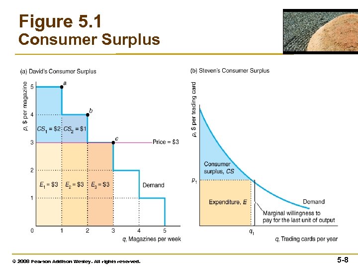Figure 5. 1 Consumer Surplus © 2008 Pearson Addison Wesley. All rights reserved. 5 -8

Effect of a Price Change on Consumer Surplus • Consumer surplus loss from a higher price. – In Figure 5. 2, as the price increases from 15 to 20, Jackie loses consumer surplus equal to areas A + B. © 2008 Pearson Addison Wesley. All rights reserved. 5 -9

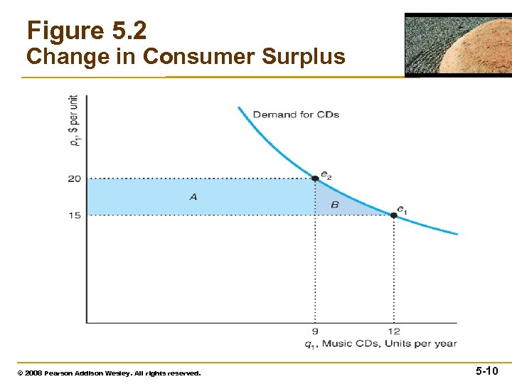Figure 5. 2 Change in Consumer Surplus © 2008 Pearson Addison Wesley. All rights reserved. 5 -10

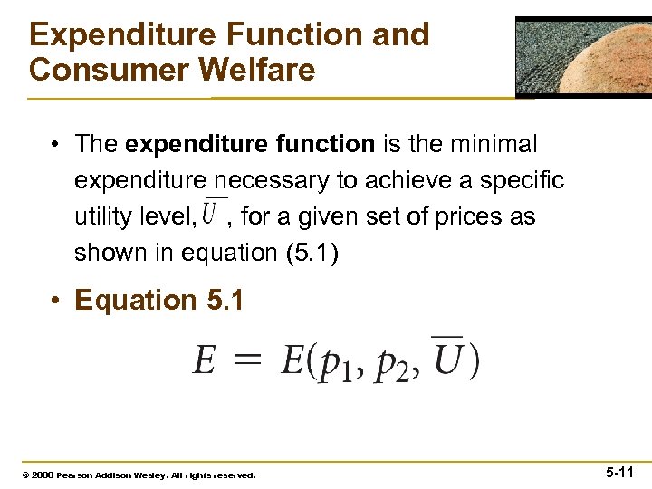Expenditure Function and Consumer Welfare • The expenditure function is the minimal expenditure necessary to achieve a specific utility level, , for a given set of prices as shown in equation (5. 1) • Equation 5. 1 © 2008 Pearson Addison Wesley. All rights reserved. 5 -11

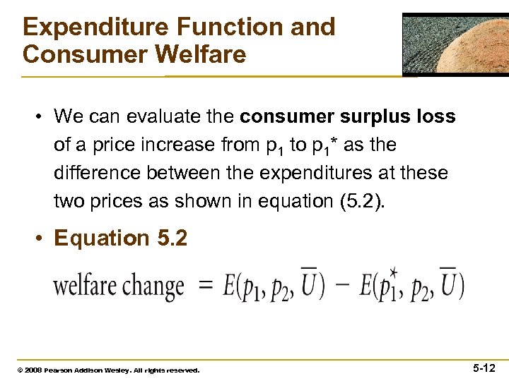Expenditure Function and Consumer Welfare • We can evaluate the consumer surplus loss of a price increase from p 1 to p 1* as the difference between the expenditures at these two prices as shown in equation (5. 2). • Equation 5. 2 © 2008 Pearson Addison Wesley. All rights reserved. 5 -12

Expenditure Function and Consumer Welfare • Compensating Variation (CV) – CV is the amount of money one would have to give a consumer to offset completely the harm from a price increase — to keep the consumer on the original indifference curve. – CV measure is the income involved in the income effect. © 2008 Pearson Addison Wesley. All rights reserved. 5 -13

Expenditure Function and Consumer Welfare • Equivalent Variation (EV) – EV is the amount of money one would have to take from a consumer to harm the consumer by as much as the price increase. It moves the consumer to the new indifference curve. © 2008 Pearson Addison Wesley. All rights reserved. 5 -14

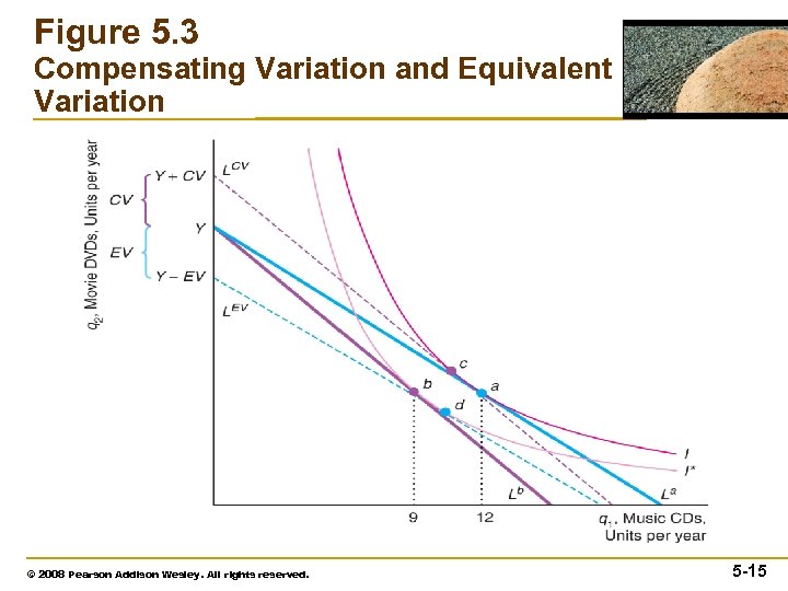Figure 5. 3 Compensating Variation and Equivalent Variation © 2008 Pearson Addison Wesley. All rights reserved. 5 -15

Comparing the Three Welfare Measures • As shown in Figure 5. 4 of a Price Increase: ΔCS: areas A + B CV : areas A + B + C EV : area A →If the good is normal, |CV| > |ΔCS| > |EV| ; →If the good is inferior, |CV| < |ΔCS| < |EV| ; © 2008 Pearson Addison Wesley. All rights reserved. 5 -16

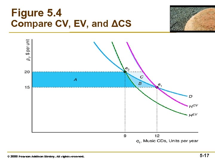Figure 5. 4 Compare CV, EV, and ΔCS © 2008 Pearson Addison Wesley. All rights reserved. 5 -17

Little Difference Between the Three Measures • According to the Slutsky equation, the uncompensated elasticity of demand, e , equals the compensated elasticity of demand, e*, minus the budget share of the good, q , times the income elasticity, x. (equation 4. 9) • The smaller the income elasticity or budget share, the closer the three welfare measure are to each other. © 2008 Pearson Addison Wesley. All rights reserved. 5 -18

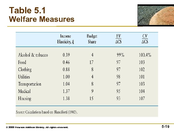Table 5. 1 Welfare Measures © 2008 Pearson Addison Wesley. All rights reserved. 5 -19

Market Consumer Surplus • Market consumer surplus is the area under the market demand curve above the market price up to the quantity consumers buy. © 2008 Pearson Addison Wesley. All rights reserved. 5 -20

Loss of Market Consumer Surplus from A Higher Price • In general, as the price increases, consumer surplus falls more, 1) the greater the initial revenues spent on the good, 2) the less elastic the demand curve. © 2008 Pearson Addison Wesley. All rights reserved. 5 -21

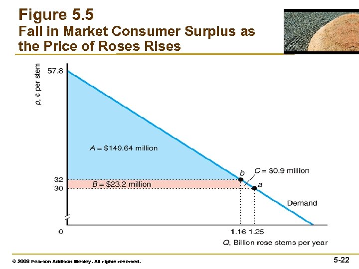Figure 5. 5 Fall in Market Consumer Surplus as the Price of Roses Rises © 2008 Pearson Addison Wesley. All rights reserved. 5 -22

Loss of a Market Consumer Surplus from A Higher Price • Higher prices cause greater consumer loss in some markets than in others. • Consumers would benefit if policymakers, before imposing a tax, considered in which market the tax would be likely to harm consumers the most. © 2008 Pearson Addison Wesley. All rights reserved. 5 -23

Effects of Government Policies on Consumer Welfare • The various consumer welfare measures are used to answer questions about the effect on consumers of government programs and other events that shift consumers’ budget constraints. © 2008 Pearson Addison Wesley. All rights reserved. 5 -24

Quotas • Consumers welfare is reduced if they cannot buy as many units of a good as they want. • Firms and government frequently limit how much of a good one can buy by setting a quota. © 2008 Pearson Addison Wesley. All rights reserved. 5 -25

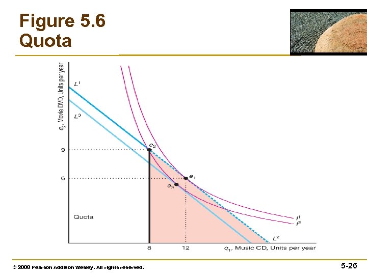Figure 5. 6 Quota © 2008 Pearson Addison Wesley. All rights reserved. 5 -26

Quota • As shown in Fig. 5. 6, the quota harms a consumer because he/she has moved from a higher indifference curve, I 1, to a lower indifference curve, I 2. • The difference between the expenditure on the original budget line and the new expenditure is this consumer’s equivalent variation. © 2008 Pearson Addison Wesley. All rights reserved. 5 -27

Food Stamps • Why cash is preferred to food stamps – Poor people who receive cash have more choices than those who receive a comparable amount of food stamps. • As shown in Fig. 5. 7, if we draw a budget line with the same slope as the original that is tangent to I 2, we can calculate the equivalent variation. © 2008 Pearson Addison Wesley. All rights reserved. 5 -28

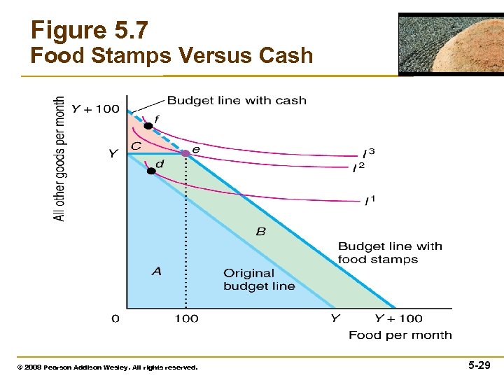Figure 5. 7 Food Stamps Versus Cash © 2008 Pearson Addison Wesley. All rights reserved. 5 -29

Child-Care Subsidies • Would a price subsidy or a lump-sum subsidy provide greater benefit to recipients for a given government expenditure? • Fig. 5. 8 shows that the family is better off with the lump sum than with the price subsidy of child-care. © 2008 Pearson Addison Wesley. All rights reserved. 5 -30

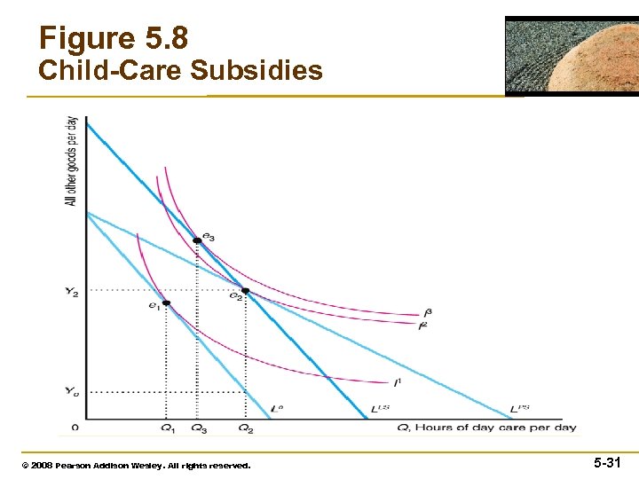Figure 5. 8 Child-Care Subsidies © 2008 Pearson Addison Wesley. All rights reserved. 5 -31

主要國家實際每週 時 • 我國自 2001年起每週實際 時明顯下降，由 2000年之43. 6小時降至 2006年之41. 6小時，低於韓國之44. 2小時、新加坡之46. 2小時(25人以上事 業單位)及香港之47小時，但仍高於日本之35. 4小時及美國之33. 9小時。 • 洛桑管理學院(IMD) 2007年全球競爭力報告中指出，2006年各國實際 年 作時數最長的前四名依序為韓國2, 439小時、墨西哥 2, 385小時、香港 2, 348小時、印度 2, 277小時，皆高於我國之2, 256小時（事實上根據行政院 主計處統計，我國年 時為月平均 時180. 8*12個月=2, 170小時）。 資料來源：行政院勞 委員會統計處 各國法定 時與實際 時比較 © 2008 Pearson Addison Wesley. All rights reserved. 5 -32

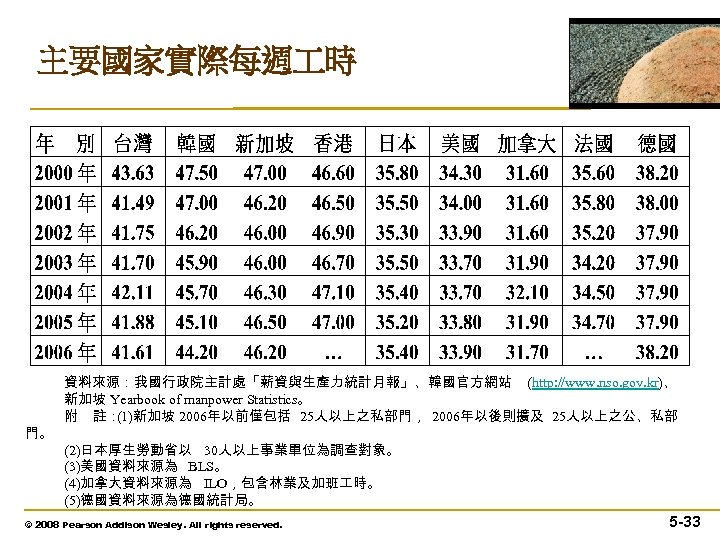主要國家實際每週 時 門。 資料來源：我國行政院主計處「薪資與生產力統計月報」、韓國官方網站 (http: //www. nso. gov. kr)、 新加坡 Yearbook of manpower Statistics。 附 註： (1)新加坡 2006年以前僅包括 25人以上之私部門， 2006年以後則擴及 25人以上之公、私部 (2)日本厚生勞動省以 30人以上事業單位為調查對象。 (3)美國資料來源為 BLS。 (4)加拿大資料來源為 ILO，包含林業及加班 時。 (5)德國資料來源為德國統計局。 © 2008 Pearson Addison Wesley. All rights reserved. 5 -33

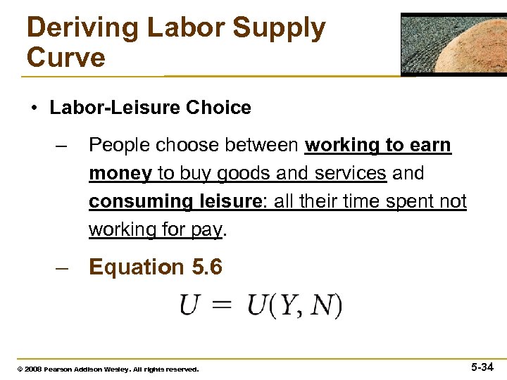Deriving Labor Supply Curve • Labor-Leisure Choice – People choose between working to earn money to buy goods and services and consuming leisure: all their time spent not working for pay. – Equation 5. 6 © 2008 Pearson Addison Wesley. All rights reserved. 5 -34

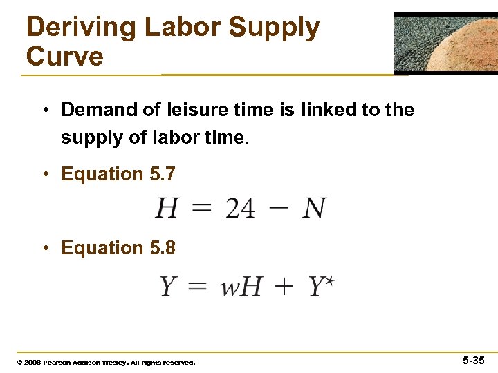Deriving Labor Supply Curve • Demand of leisure time is linked to the supply of labor time. • Equation 5. 7 • Equation 5. 8 © 2008 Pearson Addison Wesley. All rights reserved. 5 -35

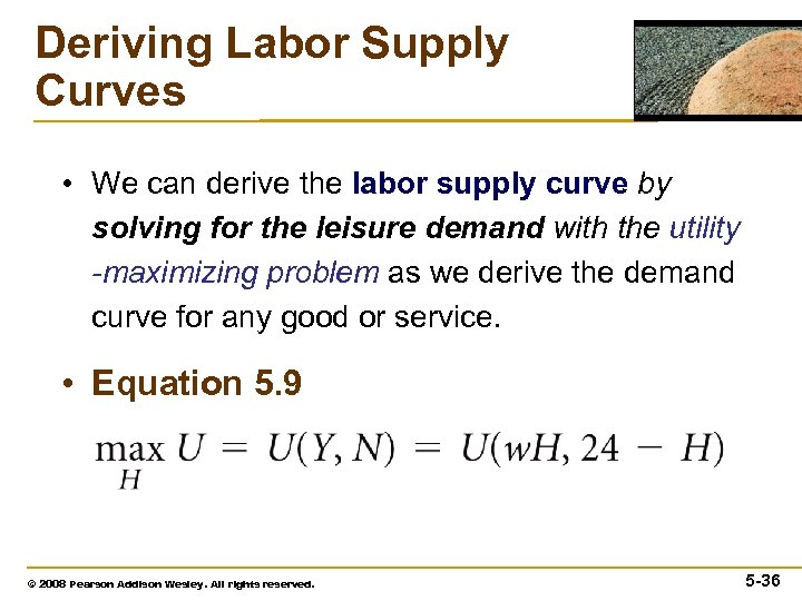Deriving Labor Supply Curves • We can derive the labor supply curve by solving for the leisure demand with the utility -maximizing problem as we derive the demand curve for any good or service. • Equation 5. 9 © 2008 Pearson Addison Wesley. All rights reserved. 5 -36

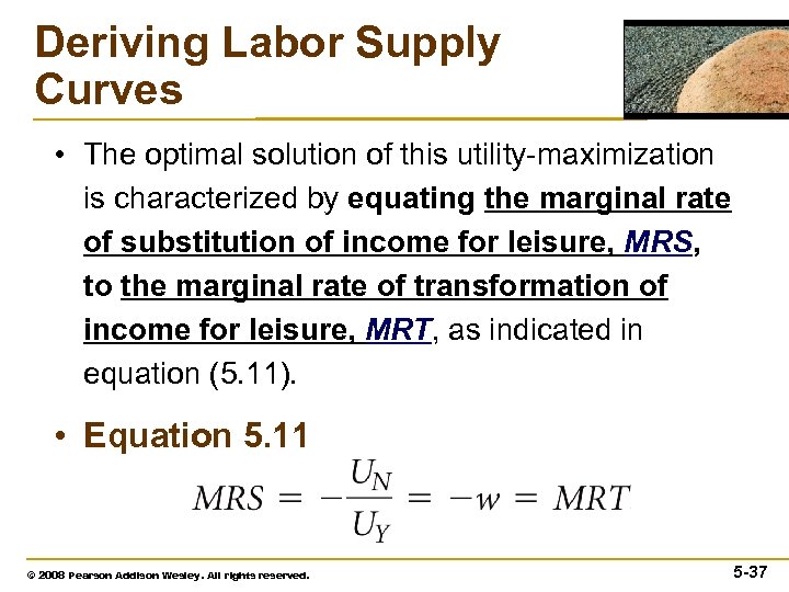Deriving Labor Supply Curves • The optimal solution of this utility-maximization is characterized by equating the marginal rate of substitution of income for leisure, MRS, to the marginal rate of transformation of income for leisure, MRT, as indicated in equation (5. 11). • Equation 5. 11 © 2008 Pearson Addison Wesley. All rights reserved. 5 -37

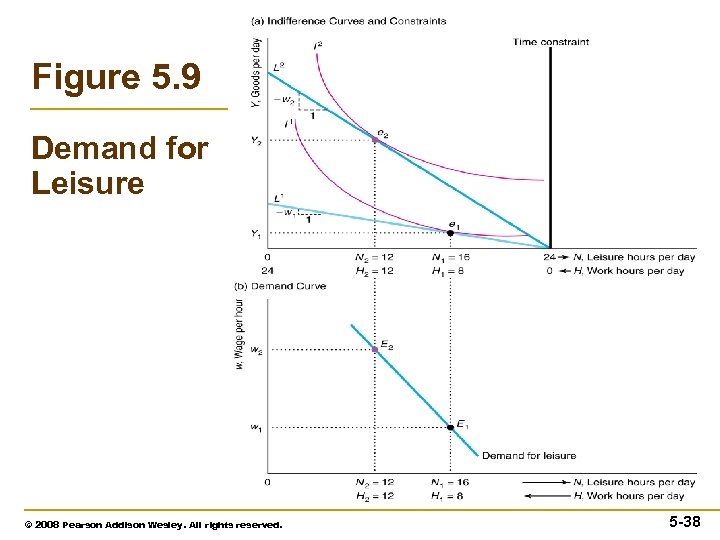Figure 5. 9 Demand for Leisure © 2008 Pearson Addison Wesley. All rights reserved. 5 -38

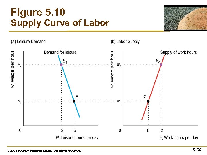Figure 5. 10 Supply Curve of Labor © 2008 Pearson Addison Wesley. All rights reserved. 5 -39

Income and Substitution Effects • When leisure is a normal good, the substitution and income effects work in opposite directions, so whether leisure demand increases or not depends on which effect is larger. • If leisure is an inferior good, both the substitution and income effect work in the same direction, a wage increase unambiguously causes the hours worked to rise. © 2008 Pearson Addison Wesley. All rights reserved. 5 -40

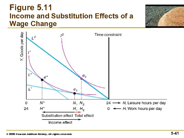Figure 5. 11 Income and Substitution Effects of a Wage Change © 2008 Pearson Addison Wesley. All rights reserved. 5 -41

Shape of the Labor Supply Curve • The labor supply curve can slope upward, bend backward, or have sections with both properties depending on the income elasticity of leisure. • At low wages, the substitution effect—work more hours—dominates the income effect— work fewer hours—while the opposite occurs at higher wages. © 2008 Pearson Addison Wesley. All rights reserved. 5 -42

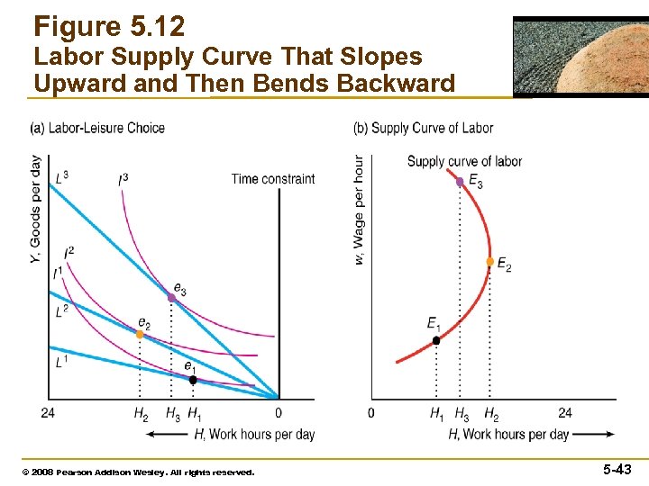Figure 5. 12 Labor Supply Curve That Slopes Upward and Then Bends Backward © 2008 Pearson Addison Wesley. All rights reserved. 5 -43

Income Tax and Labor Supply • Taxes on earnings are an unattractive way of collecting money for the government if supply curves are upward sloping, because the taxes cause people to work fewer hours, reducing the amount of goods that society produces and raising less tax revenue than if the supply curve were vertical or backward bending. © 2008 Pearson Addison Wesley. All rights reserved. 5 -44

Income Tax and Labor Supply • If the worker is in the backward-bending section of the labor supply curve, the relationship between the marginal tax rate and tax revenue is bell-shaped, as in Fig. 5. 13. © 2008 Pearson Addison Wesley. All rights reserved. 5 -45

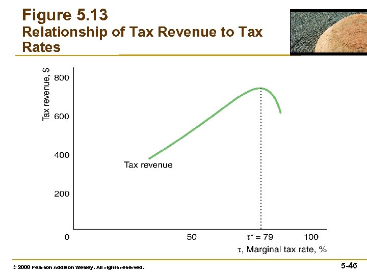Figure 5. 13 Relationship of Tax Revenue to Tax Rates © 2008 Pearson Addison Wesley. All rights reserved. 5 -46

Income Tax and Labor Supply • At first, if the tax rate rises a little more, tax revenue must rise even higher, for two reasons. 1) The government collects a larger percentage of every dollar earned because the tax rate is higher. 2) Employees work more hours as the tax rate rises because workers are in the backwardbending section. © 2008 Pearson Addison Wesley. All rights reserved. 5 -47

Income Tax and Labor Supply • As the tax rate rises far enough, the workers are in the upward-sloping section. • In the upward-sloping section, an increase in the tax rate reduces the number of hours worked. • When the reduction in hours worked more than offsets the gain from the higher tax rate, so tax revenue falls. © 2008 Pearson Addison Wesley. All rights reserved. 5 -48