Varian_Chapter05_Choice_mod.ppt
- Количество слайдов: 77
 Chapter Five Choice
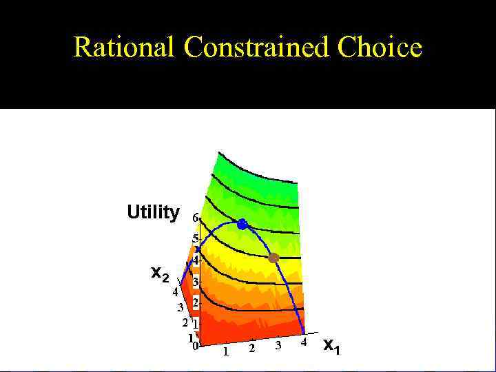
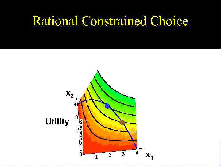
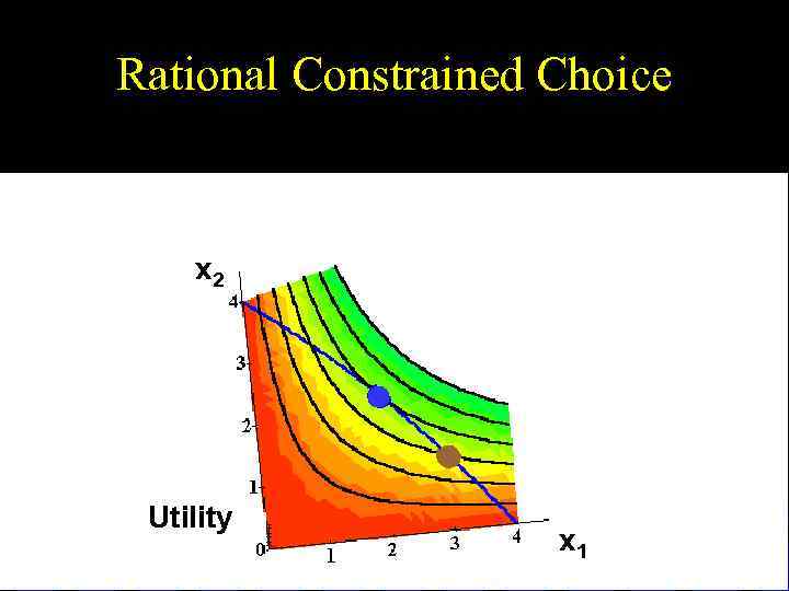
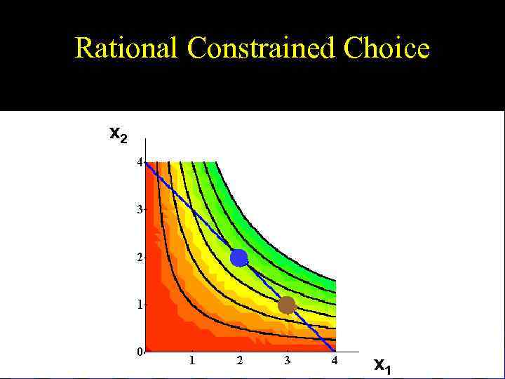
 Economic Rationality u The principal behavioral postulate is that a decisionmaker chooses its most preferred alternative from those available to it. u The available choices constitute the choice set. u How is the most preferred bundle in the choice set located?
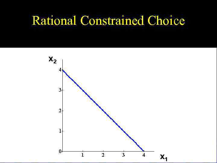 Rational Constrained Choice x 2 x 1
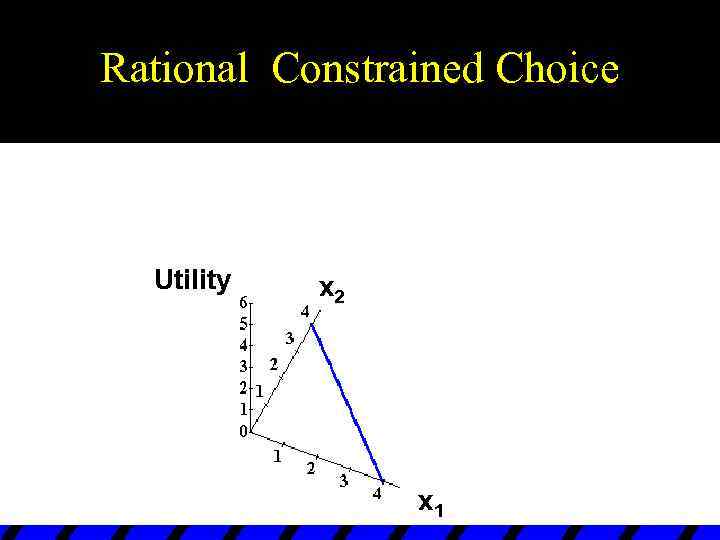 Rational Constrained Choice Utility x 2 x 1
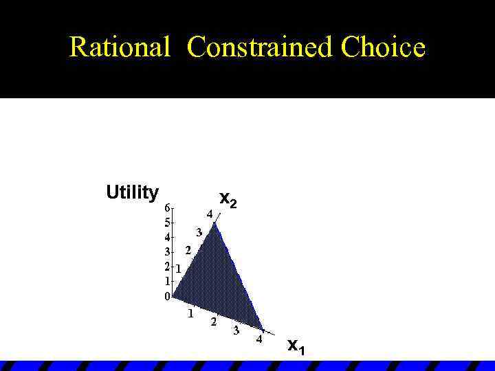 Rational Constrained Choice Utility x 2 x 1
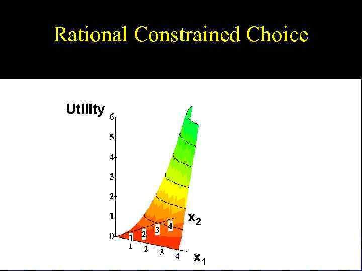 Rational Constrained Choice Utility x 2 x 1
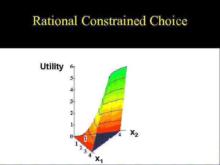 Rational Constrained Choice Utility x 2 x 1
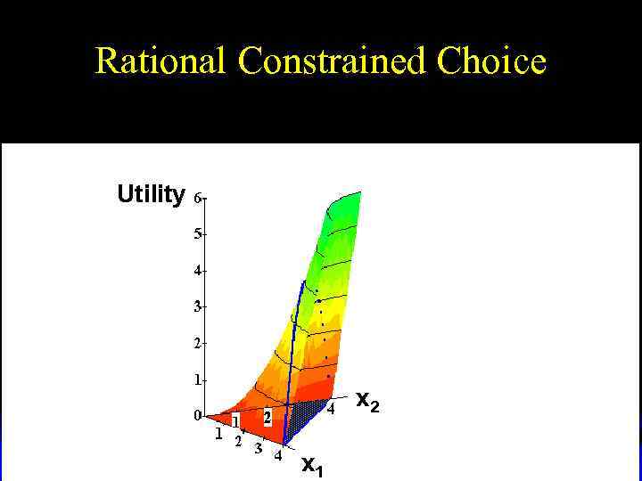 Rational Constrained Choice Utility x 2 x 1
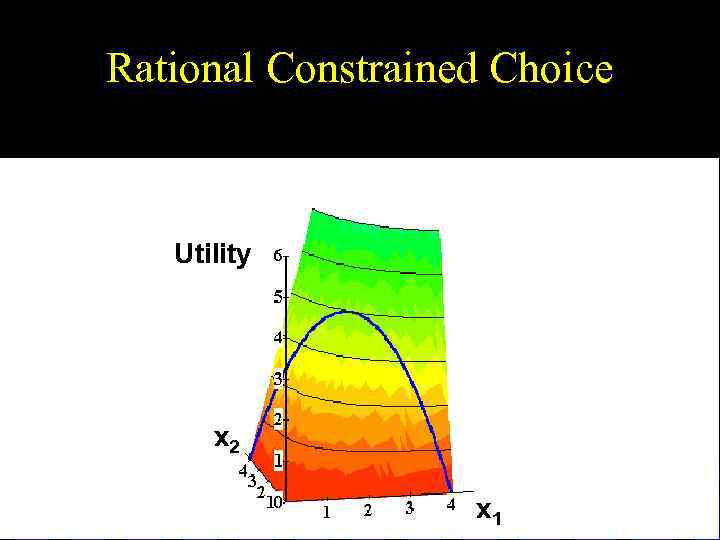 Rational Constrained Choice Utility x 2 x 1
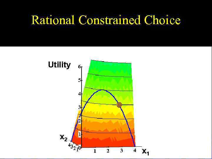 Rational Constrained Choice Utility x 2 x 1
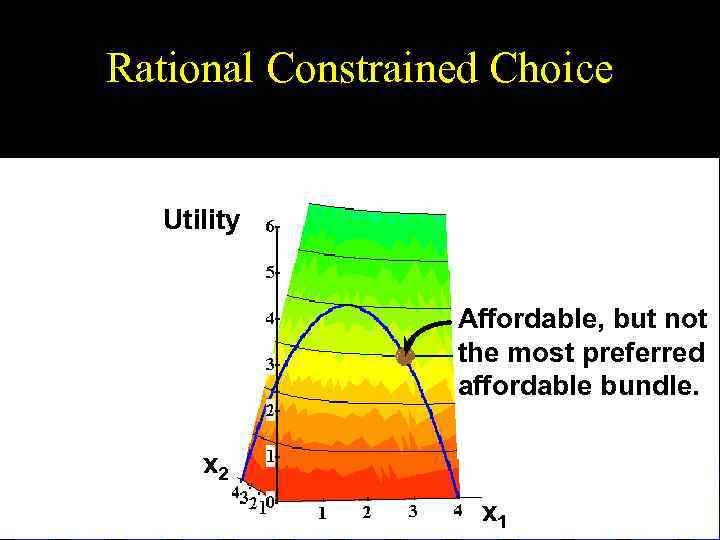 Rational Constrained Choice Utility Affordable, but not the most preferred affordable bundle. x 2 x 1
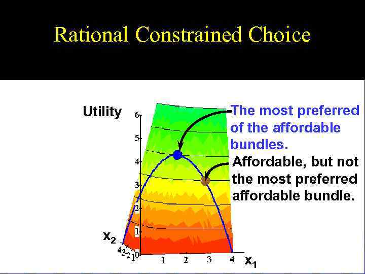 Rational Constrained Choice Utility The most preferred of the affordable bundles. Affordable, but not the most preferred affordable bundle. x 2 x 1
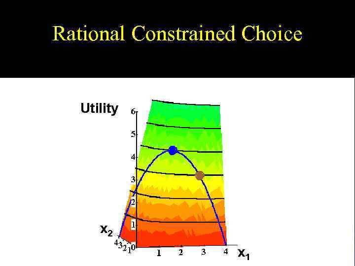 Rational Constrained Choice Utility x 2 x 1
 Rational Constrained Choice Utility x 2 x 1
 Rational Constrained Choice x 2 Utility x 1
 Rational Constrained Choice x 2 Utility x 1
 Rational Constrained Choice x 2 x 1
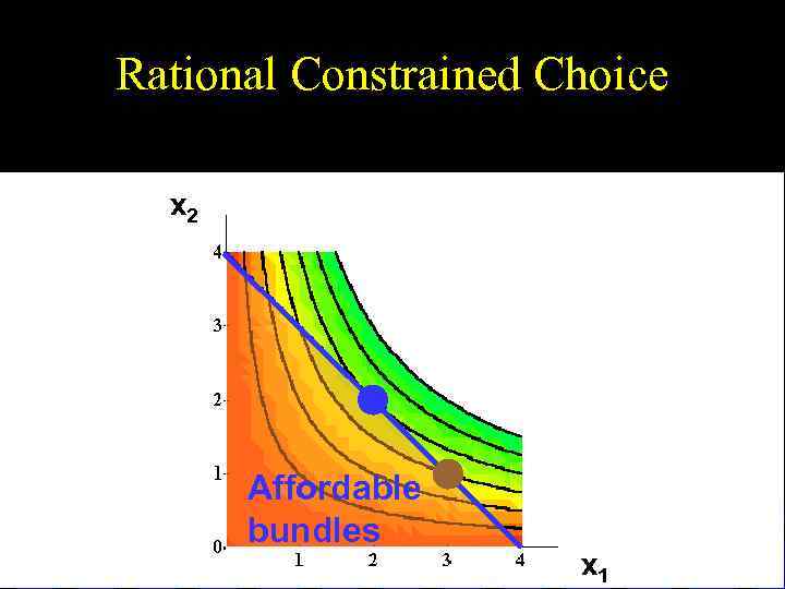 Rational Constrained Choice x 2 Affordable bundles x 1
 Rational Constrained Choice x 2 Affordable bundles x 1
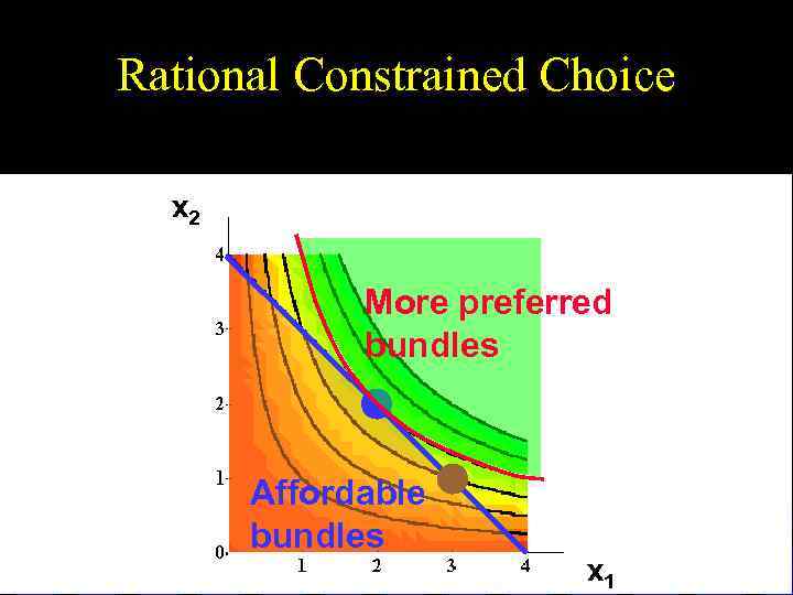 Rational Constrained Choice x 2 More preferred bundles Affordable bundles x 1
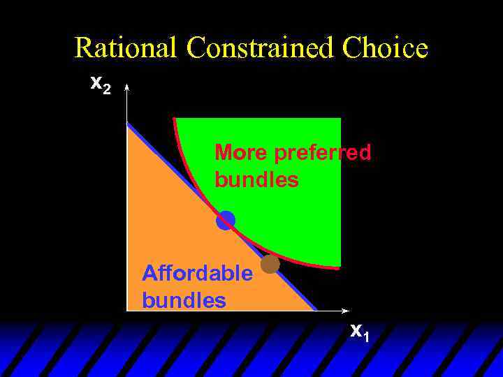 Rational Constrained Choice x 2 More preferred bundles Affordable bundles x 1
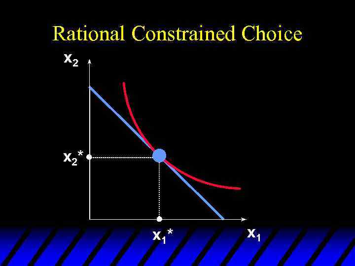 Rational Constrained Choice x 2* x 1
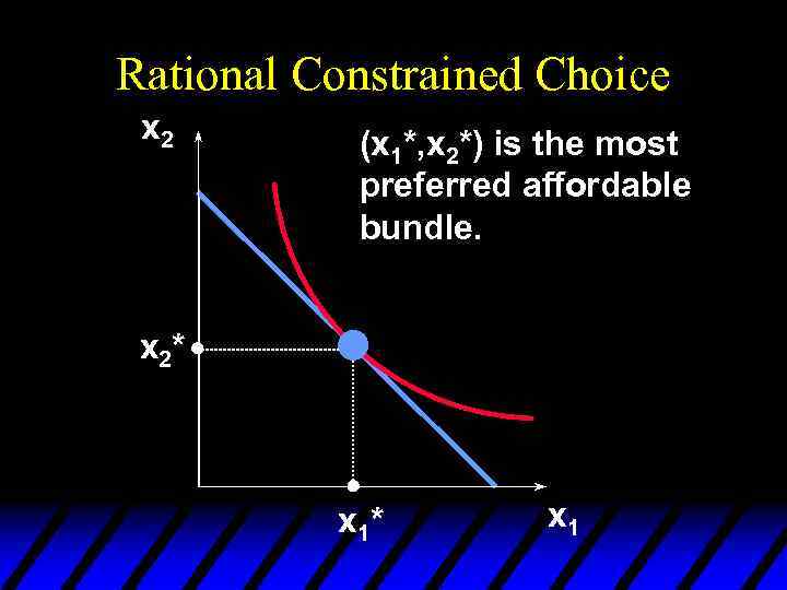 Rational Constrained Choice x 2 (x 1*, x 2*) is the most preferred affordable bundle. x 2* x 1
 Rational Constrained Choice u The most preferred affordable bundle is called the consumer’s ORDINARY DEMAND at the given prices and budget. u Ordinary demands will be denoted by x 1*(p 1, p 2, m) and x 2*(p 1, p 2, m).
 Rational Constrained Choice u When x 1* > 0 and x 2* > 0 the demanded bundle is INTERIOR. u If buying (x 1*, x 2*) costs $m then the budget is exhausted.
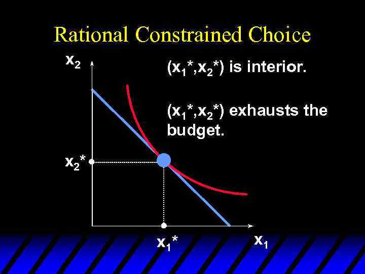 Rational Constrained Choice x 2 (x 1*, x 2*) is interior. (x 1*, x 2*) exhausts the budget. x 2* x 1
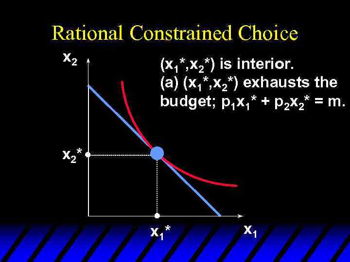 Rational Constrained Choice x 2 (x 1*, x 2*) is interior. (a) (x 1*, x 2*) exhausts the budget; p 1 x 1* + p 2 x 2* = m. x 2* x 1
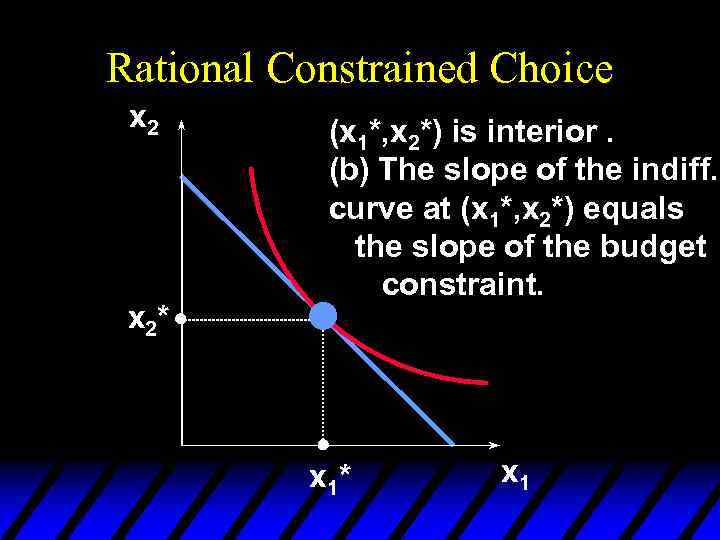 Rational Constrained Choice x 2* (x 1*, x 2*) is interior. (b) The slope of the indiff. curve at (x 1*, x 2*) equals the slope of the budget constraint. x 1* x 1
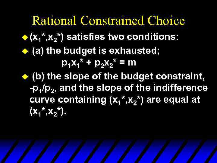 Rational Constrained Choice u (x 1*, x 2*) satisfies two conditions: u (a) the budget is exhausted; p 1 x 1* + p 2 x 2* = m u (b) the slope of the budget constraint, -p 1/p 2, and the slope of the indifference curve containing (x 1*, x 2*) are equal at (x 1*, x 2*).
 Computing Ordinary Demands u How can this information be used to locate (x 1*, x 2*) for given p 1, p 2 and m?
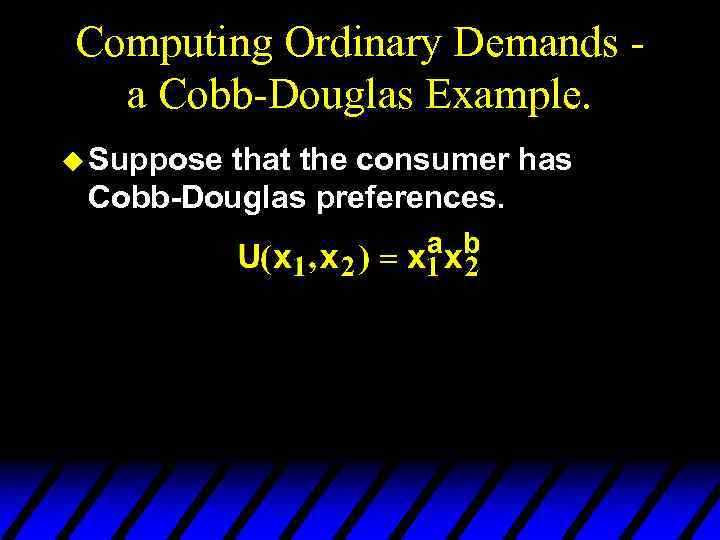 Computing Ordinary Demands a Cobb-Douglas Example. u Suppose that the consumer has Cobb-Douglas preferences.
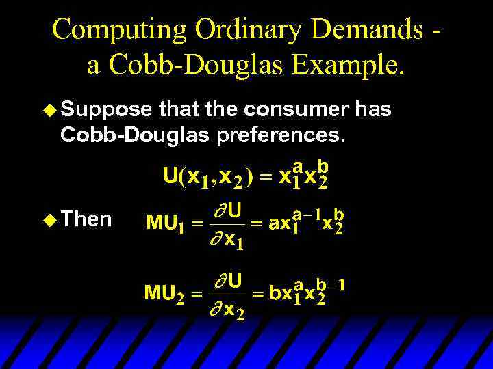 Computing Ordinary Demands a Cobb-Douglas Example. u Suppose that the consumer has Cobb-Douglas preferences. u Then
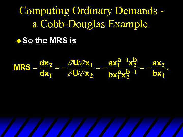 Computing Ordinary Demands a Cobb-Douglas Example. u So the MRS is
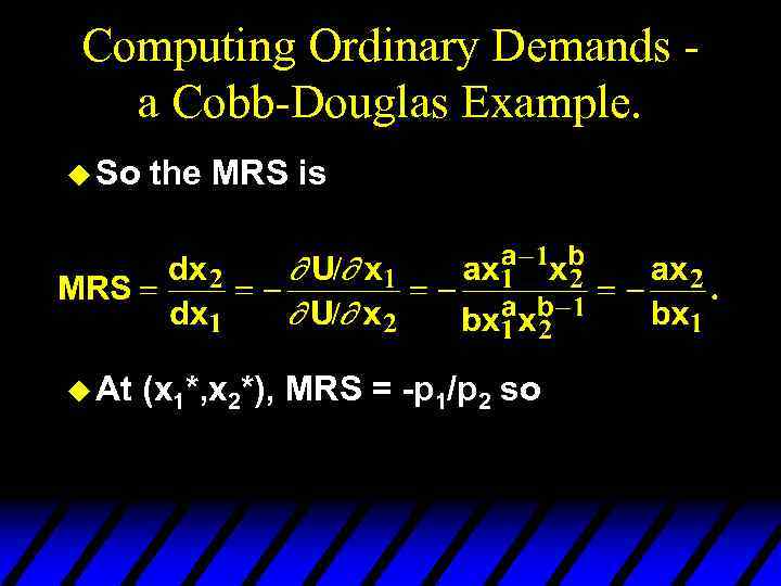 Computing Ordinary Demands a Cobb-Douglas Example. u So the MRS is u At (x 1*, x 2*), MRS = -p 1/p 2 so
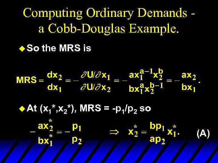 Computing Ordinary Demands a Cobb-Douglas Example. u So the MRS is u At (x 1*, x 2*), MRS = -p 1/p 2 so (A)
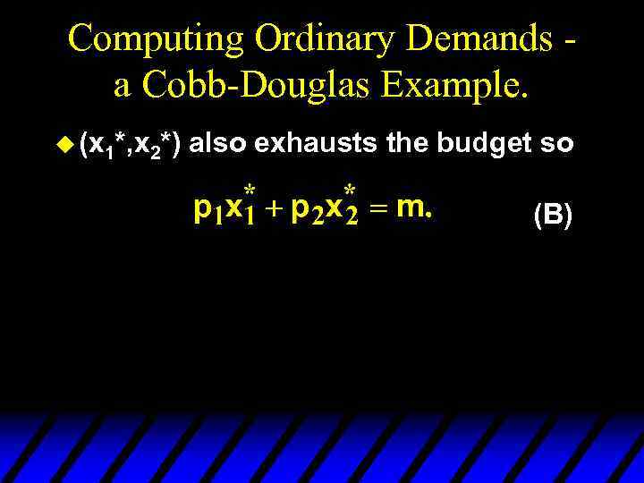 Computing Ordinary Demands a Cobb-Douglas Example. u (x 1*, x 2*) also exhausts the budget so (B)
 Computing Ordinary Demands a Cobb-Douglas Example. u So now we know that (A) (B)
 Computing Ordinary Demands a Cobb-Douglas Example. u So now we know that (A) Substitute (B)
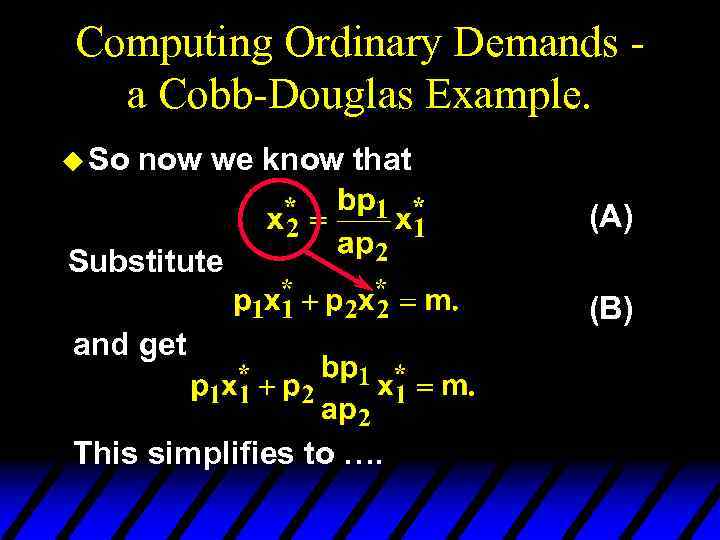 Computing Ordinary Demands a Cobb-Douglas Example. u So now we know that (A) Substitute and get This simplifies to …. (B)
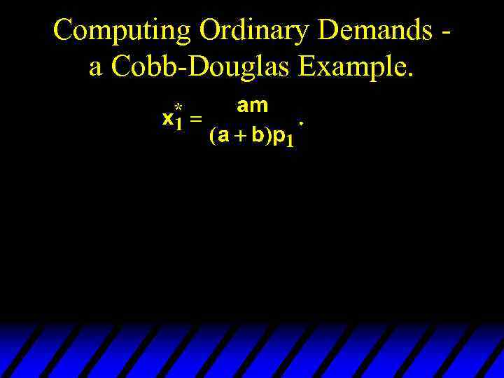 Computing Ordinary Demands a Cobb-Douglas Example.
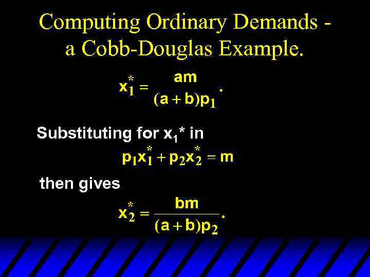 Computing Ordinary Demands a Cobb-Douglas Example. Substituting for x 1* in then gives
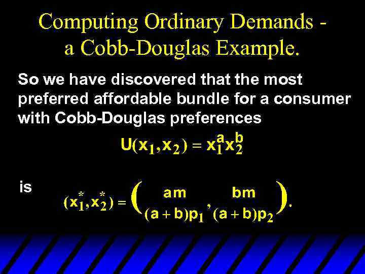 Computing Ordinary Demands a Cobb-Douglas Example. So we have discovered that the most preferred affordable bundle for a consumer with Cobb-Douglas preferences is
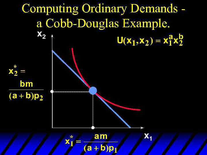 Computing Ordinary Demands a Cobb-Douglas Example. x 2 x 1
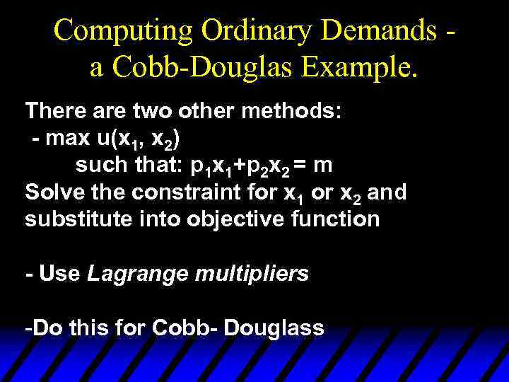 Computing Ordinary Demands a Cobb-Douglas Example. There are two other methods: - max u(x 1, x 2) such that: p 1 x 1+p 2 x 2 = m Solve the constraint for x 1 or x 2 and substitute into objective function - Use Lagrange multipliers -Do this for Cobb- Douglass
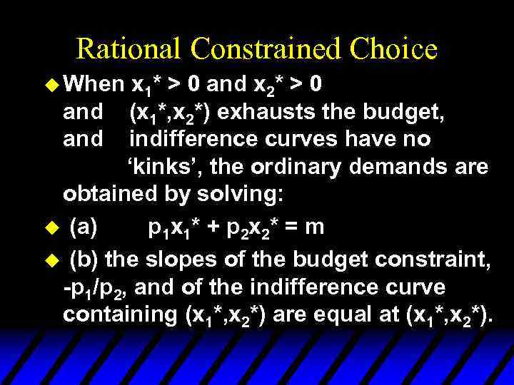 Rational Constrained Choice u When x 1* > 0 and x 2* > 0 and (x 1*, x 2*) exhausts the budget, and indifference curves have no ‘kinks’, the ordinary demands are obtained by solving: u (a) p 1 x 1* + p 2 x 2* = m u (b) the slopes of the budget constraint, -p 1/p 2, and of the indifference curve containing (x 1*, x 2*) are equal at (x 1*, x 2*).
 Rational Constrained Choice u But what if x 1* = 0? u Or if x 2* = 0? u If either x 1* = 0 or x 2* = 0 then the ordinary demand (x 1*, x 2*) is at a corner solution to the problem of maximizing utility subject to a budget constraint.
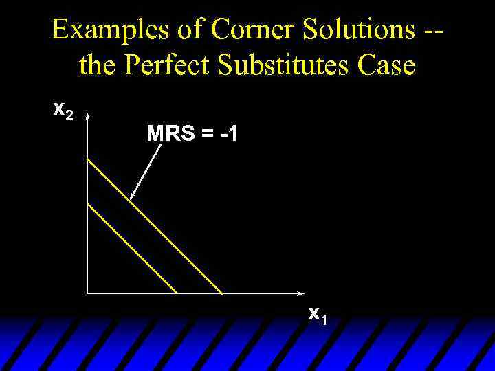 Examples of Corner Solutions -the Perfect Substitutes Case x 2 MRS = -1 x 1
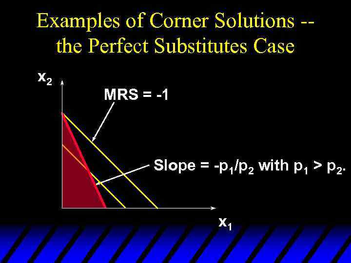 Examples of Corner Solutions -the Perfect Substitutes Case x 2 MRS = -1 Slope = -p 1/p 2 with p 1 > p 2. x 1
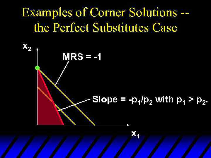 Examples of Corner Solutions -the Perfect Substitutes Case x 2 MRS = -1 Slope = -p 1/p 2 with p 1 > p 2. x 1
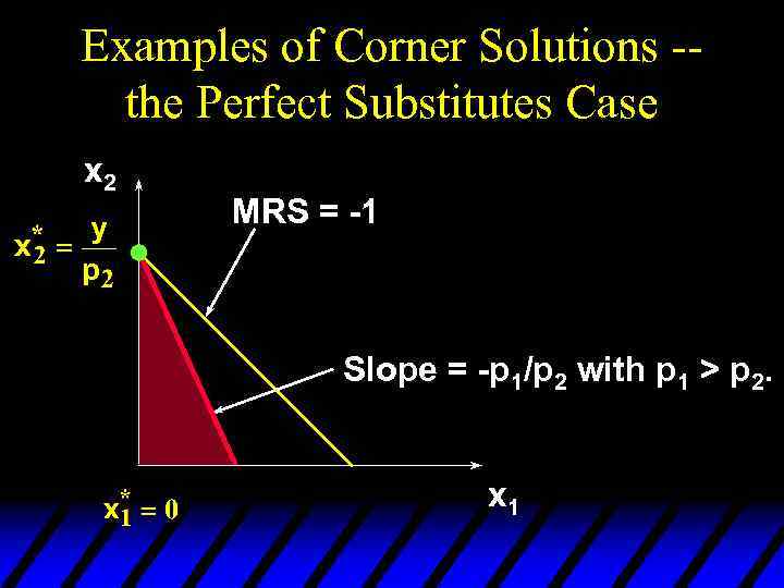 Examples of Corner Solutions -the Perfect Substitutes Case x 2 MRS = -1 Slope = -p 1/p 2 with p 1 > p 2. x 1
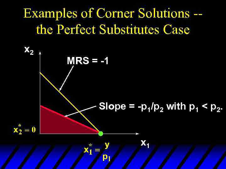 Examples of Corner Solutions -the Perfect Substitutes Case x 2 MRS = -1 Slope = -p 1/p 2 with p 1 < p 2. x 1
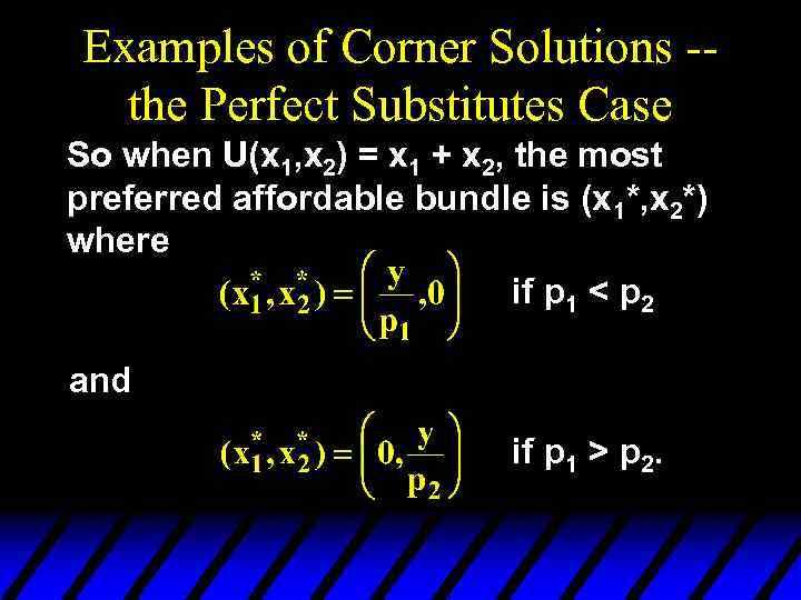 Examples of Corner Solutions -the Perfect Substitutes Case So when U(x 1, x 2) = x 1 + x 2, the most preferred affordable bundle is (x 1*, x 2*) where if p 1 < p 2 and if p 1 > p 2.
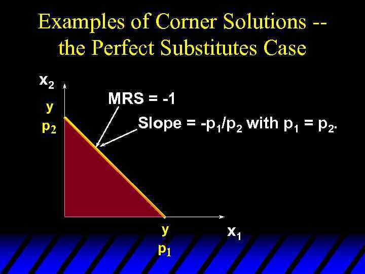 Examples of Corner Solutions -the Perfect Substitutes Case x 2 MRS = -1 Slope = -p 1/p 2 with p 1 = p 2. x 1
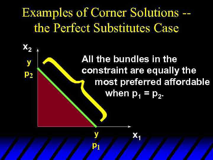 Examples of Corner Solutions -the Perfect Substitutes Case x 2 All the bundles in the constraint are equally the most preferred affordable when p 1 = p 2. x 1
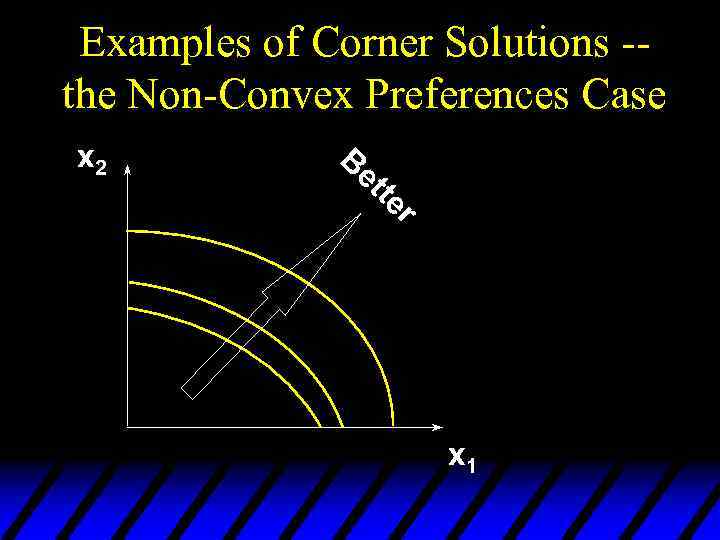 Examples of Corner Solutions -the Non-Convex Preferences Case x 2 B et te r x 1
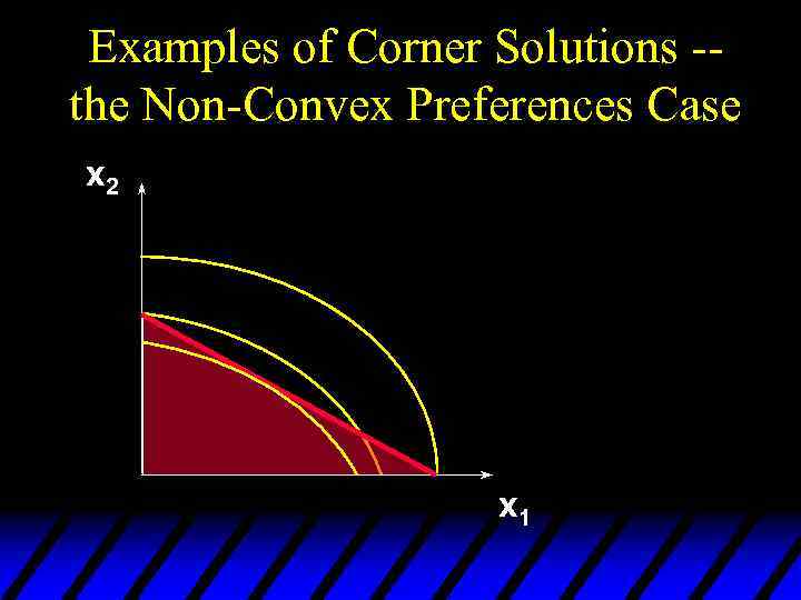 Examples of Corner Solutions -the Non-Convex Preferences Case x 2 x 1
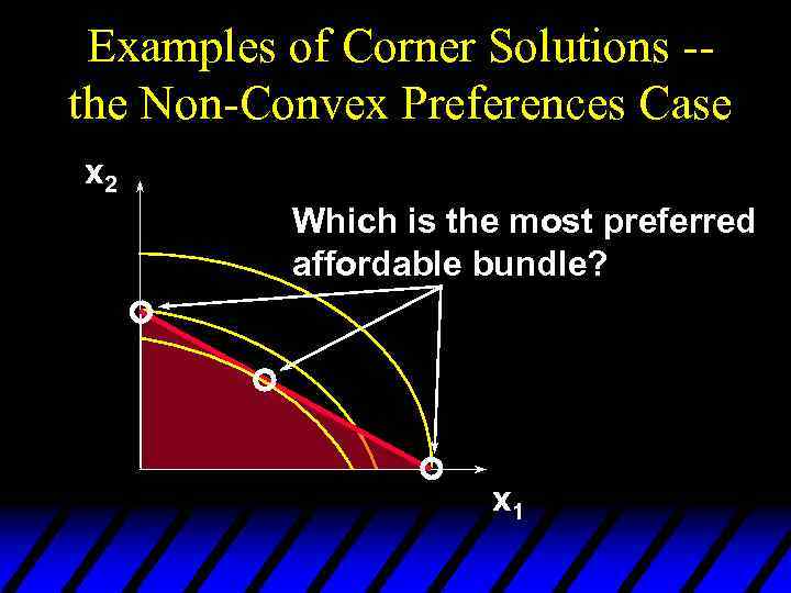 Examples of Corner Solutions -the Non-Convex Preferences Case x 2 Which is the most preferred affordable bundle? x 1
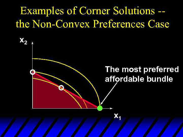 Examples of Corner Solutions -the Non-Convex Preferences Case x 2 The most preferred affordable bundle x 1
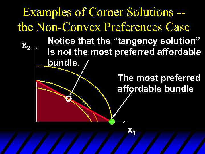 Examples of Corner Solutions -the Non-Convex Preferences Case x 2 Notice that the “tangency solution” is not the most preferred affordable bundle. The most preferred affordable bundle x 1
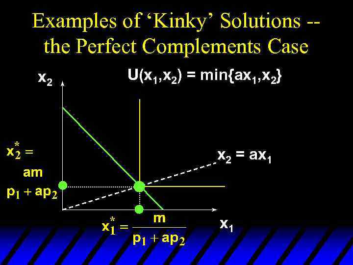
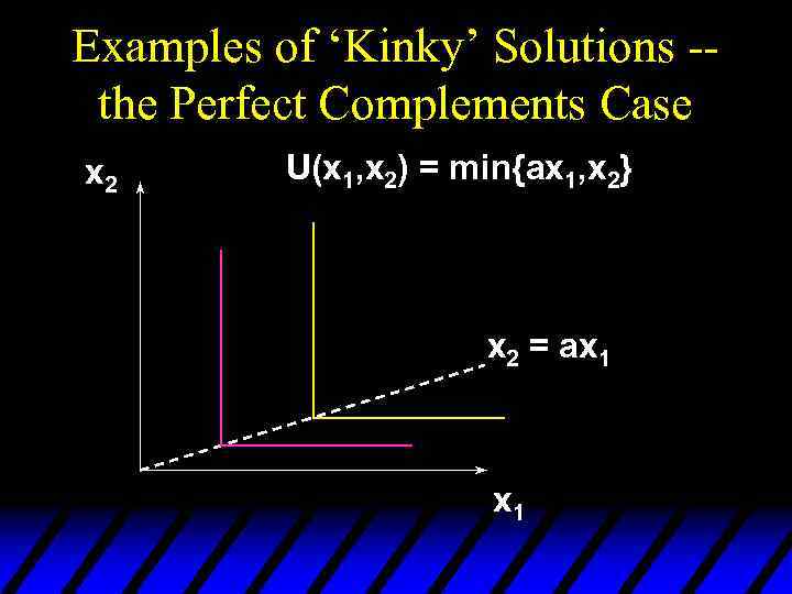 Examples of ‘Kinky’ Solutions -the Perfect Complements Case x 2 U(x 1, x 2) = min{ax 1, x 2} x 2 = ax 1
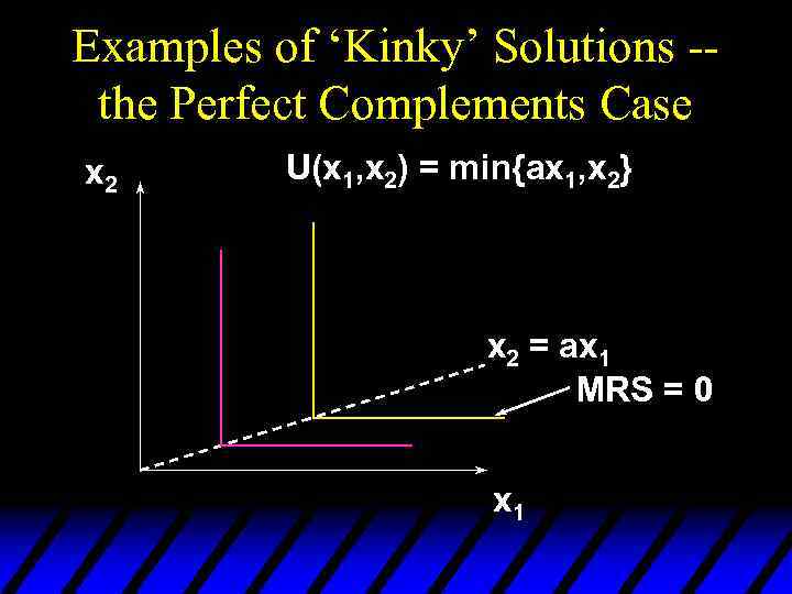 Examples of ‘Kinky’ Solutions -the Perfect Complements Case x 2 U(x 1, x 2) = min{ax 1, x 2} x 2 = ax 1 MRS = 0 x 1
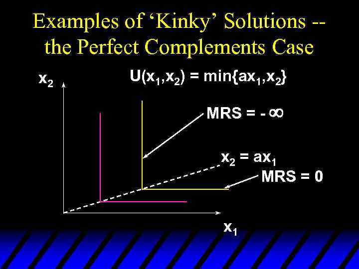 Examples of ‘Kinky’ Solutions -the Perfect Complements Case x 2 U(x 1, x 2) = min{ax 1, x 2} MRS = - x 2 = ax 1 MRS = 0 x 1
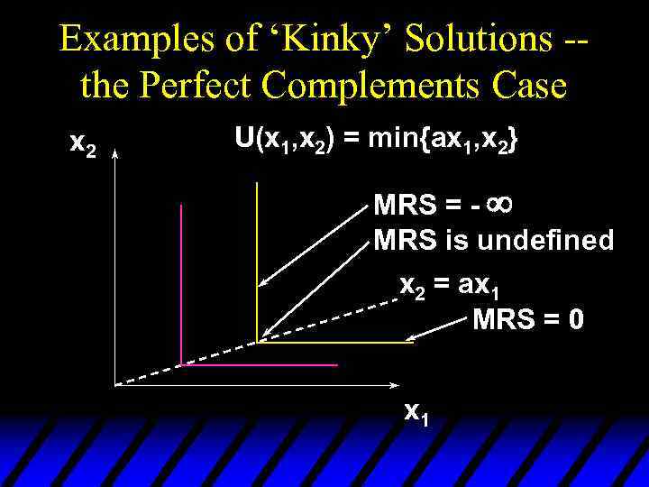 Examples of ‘Kinky’ Solutions -the Perfect Complements Case x 2 U(x 1, x 2) = min{ax 1, x 2} MRS = - MRS is undefined x 2 = ax 1 MRS = 0 x 1
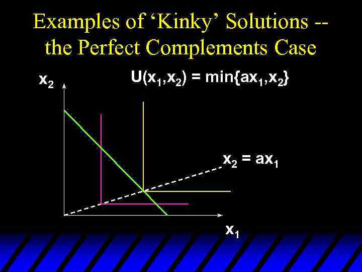 Examples of ‘Kinky’ Solutions -the Perfect Complements Case x 2 U(x 1, x 2) = min{ax 1, x 2} x 2 = ax 1
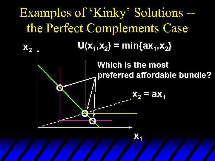 Examples of ‘Kinky’ Solutions -the Perfect Complements Case x 2 U(x 1, x 2) = min{ax 1, x 2} Which is the most preferred affordable bundle? x 2 = ax 1
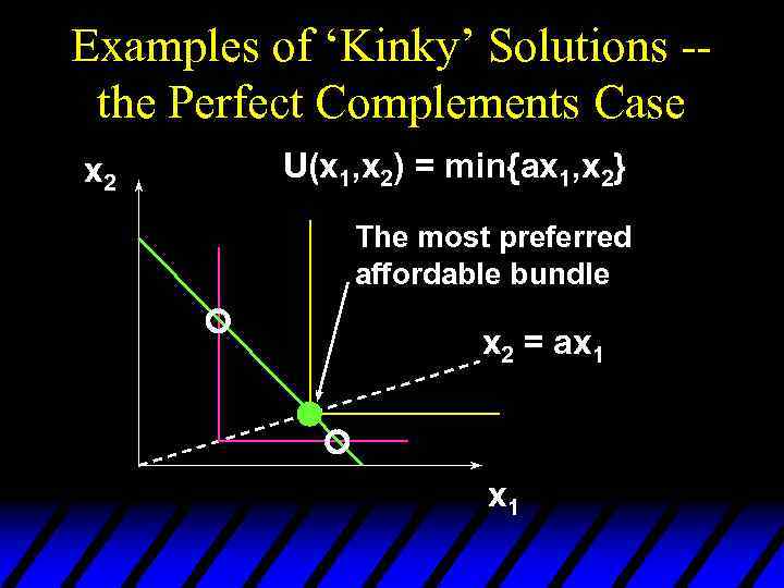 Examples of ‘Kinky’ Solutions -the Perfect Complements Case x 2 U(x 1, x 2) = min{ax 1, x 2} The most preferred affordable bundle x 2 = ax 1
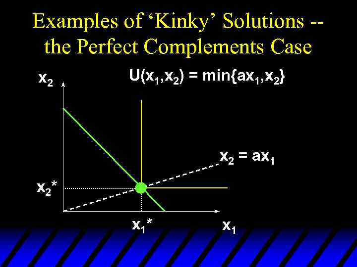 Examples of ‘Kinky’ Solutions -the Perfect Complements Case x 2 U(x 1, x 2) = min{ax 1, x 2} x 2 = ax 1 x 2* x 1
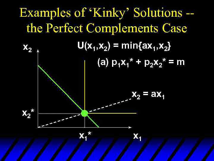 Examples of ‘Kinky’ Solutions -the Perfect Complements Case x 2 U(x 1, x 2) = min{ax 1, x 2} (a) p 1 x 1* + p 2 x 2* = m x 2 = ax 1 x 2* x 1
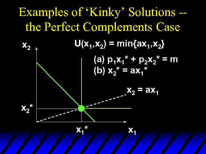 Examples of ‘Kinky’ Solutions -the Perfect Complements Case x 2 U(x 1, x 2) = min{ax 1, x 2} (a) p 1 x 1* + p 2 x 2* = m (b) x 2* = ax 1* x 2 = ax 1 x 2* x 1
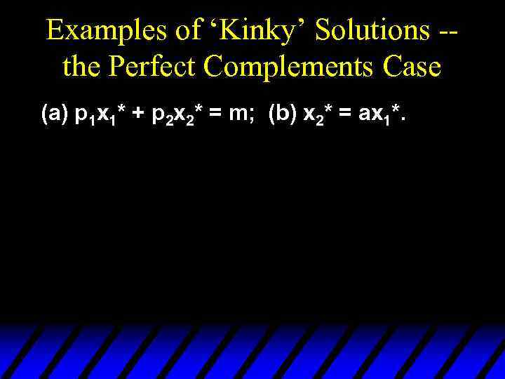 Examples of ‘Kinky’ Solutions -the Perfect Complements Case (a) p 1 x 1* + p 2 x 2* = m; (b) x 2* = ax 1*.
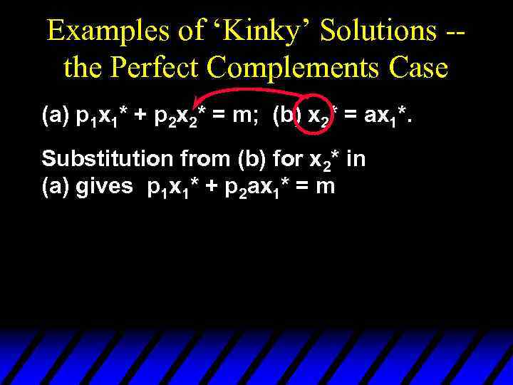 Examples of ‘Kinky’ Solutions -the Perfect Complements Case (a) p 1 x 1* + p 2 x 2* = m; (b) x 2* = ax 1*. Substitution from (b) for x 2* in (a) gives p 1 x 1* + p 2 ax 1* = m
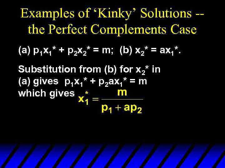 Examples of ‘Kinky’ Solutions -the Perfect Complements Case (a) p 1 x 1* + p 2 x 2* = m; (b) x 2* = ax 1*. Substitution from (b) for x 2* in (a) gives p 1 x 1* + p 2 ax 1* = m which gives
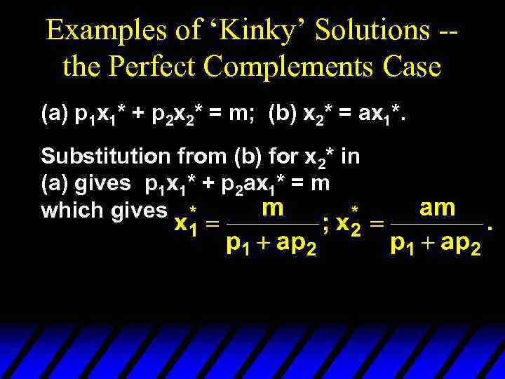 Examples of ‘Kinky’ Solutions -the Perfect Complements Case (a) p 1 x 1* + p 2 x 2* = m; (b) x 2* = ax 1*. Substitution from (b) for x 2* in (a) gives p 1 x 1* + p 2 ax 1* = m which gives
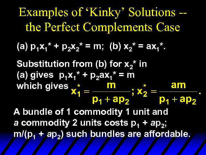 Examples of ‘Kinky’ Solutions -the Perfect Complements Case (a) p 1 x 1* + p 2 x 2* = m; (b) x 2* = ax 1*. Substitution from (b) for x 2* in (a) gives p 1 x 1* + p 2 ax 1* = m which gives A bundle of 1 commodity 1 unit and a commodity 2 units costs p 1 + ap 2; m/(p 1 + ap 2) such bundles are affordable.
 Examples of ‘Kinky’ Solutions -the Perfect Complements Case x 2 U(x 1, x 2) = min{ax 1, x 2} x 2 = ax 1
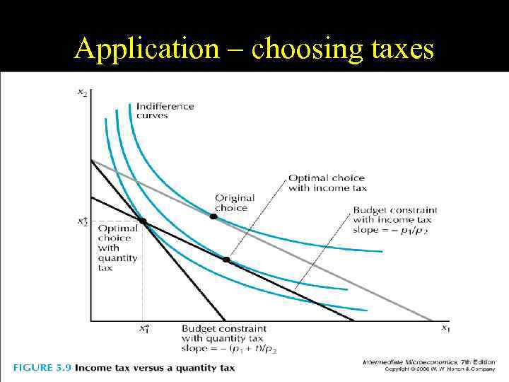
 Application – choosing taxes Quantity vs. Income tax
 Application – choosing taxes


