ed06c80729e254bdce09f64782b41bda.ppt
- Количество слайдов: 52
 Chapter Fifteen Factor Markets and Vertical Integration
 Topics § Competitive Factor Market. § Effect of Monopolies on Factor Markets. § Monopsony. § Vertical Integration. © 2009 Pearson Addison-Wesley. All rights reserved. 2
 Introductory Definitions § vertically integrated - describing a firm that participates in more than one successive stage of the production or distribution of goods or services. § monopsony - the only buyer of a good in a given market. © 2009 Pearson Addison-Wesley. All rights reserved. 3
 Short-Run Factor Demand of a Firm § A profit-maximizing firm’s demand for a factor of production is downward sloping. § In the short run, a firm has a fixed amount of capital: w. K w and can vary the number of workers, L, it employs. © 2009 Pearson Addison-Wesley. All rights reserved. 4
 Short-Run Factor Demand of a Firm (cont). § marginal revenue product of labor (MRPL) - the extra revenue from hiring one more worker: MRPL = MR. MPL © 2009 Pearson Addison-Wesley. All rights reserved. 5
 Short-Run Factor Demand of a Firm (cont). § The firm maximizes its profit by hiring workers until the marginal revenue product of the last worker exactly equals the marginal cost of employing that worker, which is the wage: MRPL = w © 2009 Pearson Addison-Wesley. All rights reserved. 6
 Short-Run Factor Demand of a Firm (cont). § A competitive firm faces an infinitely elastic demand for its output at the market price, p, so: MR = p w and MRPL = p. MPL © 2009 Pearson Addison-Wesley. All rights reserved. 7
 Short-Run Factor Demand of a Firm (cont). § The competitive firm hires labor to the point at which: MRPL = p. MPL = w § The wage line is the supply of labor the firm faces. § The marginal revenue product of labor curve, MRPL, is the firm’s demand curve for labor © 2009 Pearson Addison-Wesley. All rights reserved. 8
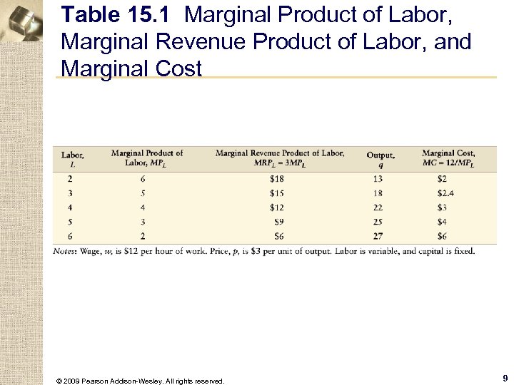 Table 15. 1 Marginal Product of Labor, Marginal Revenue Product of Labor, and Marginal Cost © 2009 Pearson Addison-Wesley. All rights reserved. 9
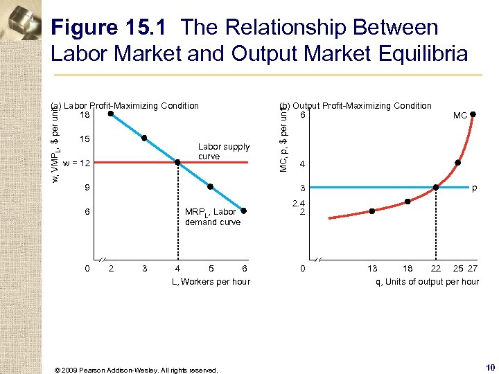 Figure 15. 1 The Relationship Between Labor Market and Output Market Equilibria 15 Labor supply curve w = 12 9 MRPL, Labor demand curve 2 3 4 5 6 L, Workers per hour © 2009 Pearson Addison-Wesley. All rights reserved. MC 4 3 6 0 (b) Output Profit-Maximizing Condition 6 MC, p, $ per unit w, VMPL, $ per unit (a) Labor Profit-Maximizing Condition 18 p 2. 4 2 0 13 18 22 25 27 q, Units of output per hour 10
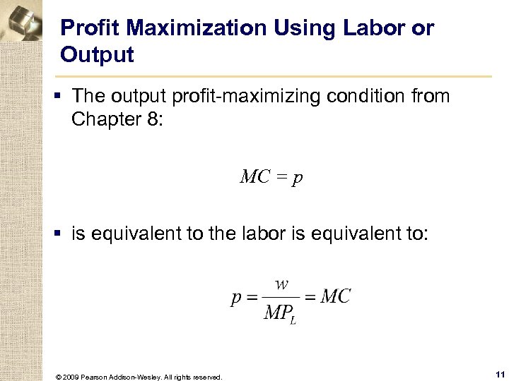 Profit Maximization Using Labor or Output § The output profit-maximizing condition from Chapter 8: MC = p § is equivalent to the labor is equivalent to: © 2009 Pearson Addison-Wesley. All rights reserved. 11
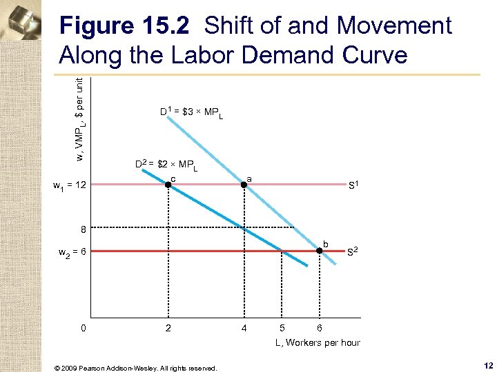 w, VMP L, $ per unit Figure 15. 2 Shift of and Movement Along the Labor Demand Curve w 1 = 12 D 1 = $3 ´ MPL D 2 = $2 ´ MPL c a S 1 8 b w 2 = 6 0 2 4 5 S 2 6 L, Workers per hour © 2009 Pearson Addison-Wesley. All rights reserved. 12
 Solved Problem 15. 1 § How does a competitive firm adjust its demand for labor when the government imposes a specific tax of τ on each unit of output? © 2009 Pearson Addison-Wesley. All rights reserved. 13
 Long-Run Factor Demand § In the long run, the firm may vary all of its inputs. w The long-run labor demand curve takes account of changes in the firm’s use of capital as the wage rises. © 2009 Pearson Addison-Wesley. All rights reserved. 14
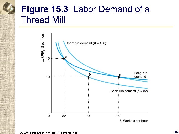 Figure 15. 3 Labor Demand of a Thread Mill © 2009 Pearson Addison-Wesley. All rights reserved. 15
 Factor Market Demand § A factor market demand curve is the sum of the factor demand curves of the various firms that use the input. w To derive the labor market demand curve, we first determine the labor demand curve for each output market and then sum across output markets to obtain the factor market demand curve. © 2009 Pearson Addison-Wesley. All rights reserved. 16
 The Marginal Revenue Product Approach. § As the factor’s price falls, each firm, taking the original market price as given, uses more of the factor to produce more output. w As the market price falls, each firm reduces its output and hence its demand for the input. A fall in an input price causes less of an increase in factor demand than would occur if the market price remained constant © 2009 Pearson Addison-Wesley. All rights reserved. 17
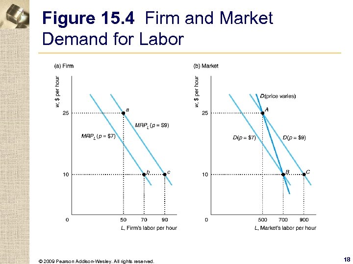 Figure 15. 4 Firm and Market Demand for Labor © 2009 Pearson Addison-Wesley. All rights reserved. 18
 An Alternative Approach. § For certain types of production functions, it is easier to determine the market demand curve by using the output profitmaximizing equation rather than the marginal revenue product approach. © 2009 Pearson Addison-Wesley. All rights reserved. 19
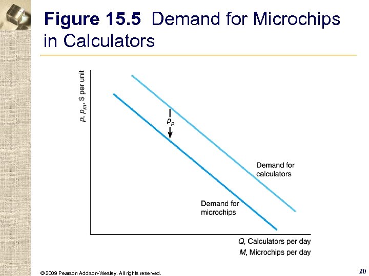 Figure 15. 5 Demand for Microchips in Calculators © 2009 Pearson Addison-Wesley. All rights reserved. 20
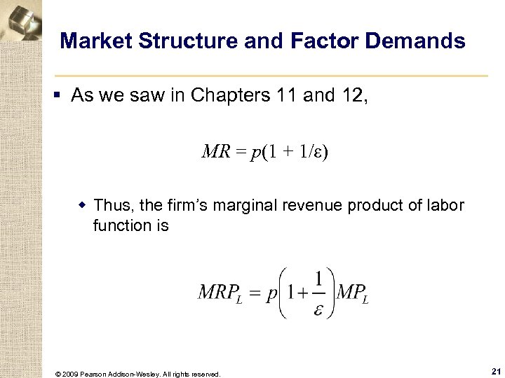 Market Structure and Factor Demands § As we saw in Chapters 11 and 12, MR = p(1 + 1/ε) w Thus, the firm’s marginal revenue product of labor function is © 2009 Pearson Addison-Wesley. All rights reserved. 21
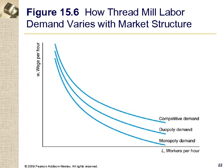 Figure 15. 6 How Thread Mill Labor Demand Varies with Market Structure © 2009 Pearson Addison-Wesley. All rights reserved. 22
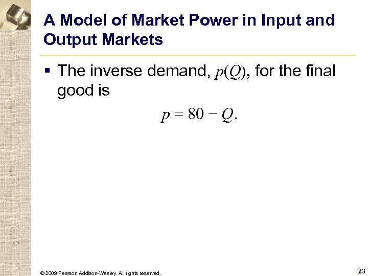 A Model of Market Power in Input and Output Markets § The inverse demand, p(Q), for the final good is p = 80 − Q. © 2009 Pearson Addison-Wesley. All rights reserved. 23
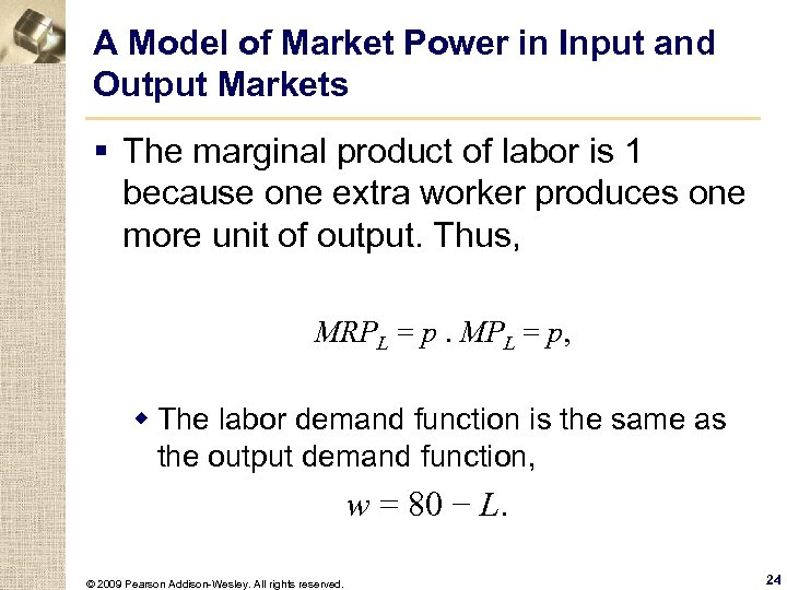 A Model of Market Power in Input and Output Markets § The marginal product of labor is 1 because one extra worker produces one more unit of output. Thus, MRPL = p. MPL = p, w The labor demand function is the same as the output demand function, w = 80 − L. © 2009 Pearson Addison-Wesley. All rights reserved. 24
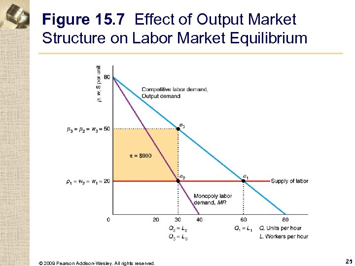 Figure 15. 7 Effect of Output Market Structure on Labor Market Equilibrium © 2009 Pearson Addison-Wesley. All rights reserved. 25
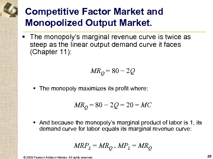 Competitive Factor Market and Monopolized Output Market. § The monopoly’s marginal revenue curve is twice as steep as the linear output demand curve it faces (Chapter 11): MRQ = 80 − 2 Q w The monopoly maximizes its profit where: MRQ = 80 − 2 Q = 20 = MC w And because the monopoly’s marginal product of labor is 1, its demand curve for labor equals its marginal revenue curve: MRPL = MRQ. MPL = MRQ © 2009 Pearson Addison-Wesley. All rights reserved. 26
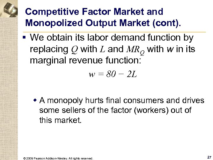 Competitive Factor Market and Monopolized Output Market (cont). § We obtain its labor demand function by replacing Q with L and MRQ with w in its marginal revenue function: w = 80 − 2 L w A monopoly hurts final consumers and drives some sellers of the factor (workers) out of this market. © 2009 Pearson Addison-Wesley. All rights reserved. 27
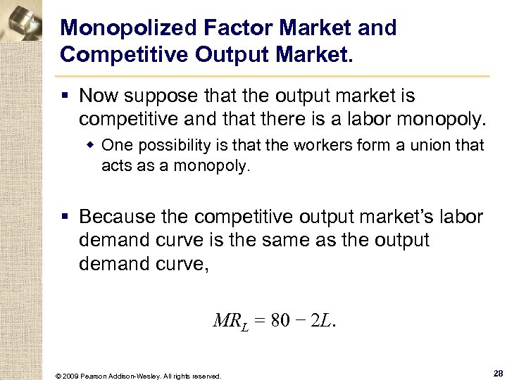 Monopolized Factor Market and Competitive Output Market. § Now suppose that the output market is competitive and that there is a labor monopoly. w One possibility is that the workers form a union that acts as a monopoly. § Because the competitive output market’s labor demand curve is the same as the output demand curve, MRL = 80 − 2 L. © 2009 Pearson Addison-Wesley. All rights reserved. 28
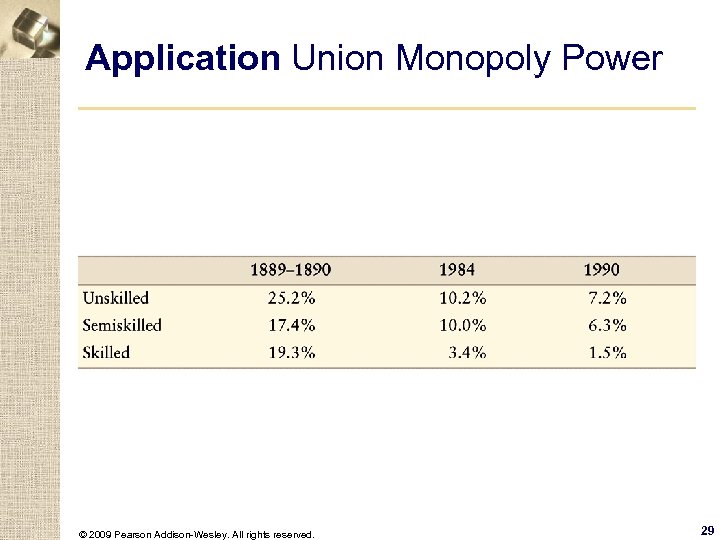 Application Union Monopoly Power © 2009 Pearson Addison-Wesley. All rights reserved. 29
 Monopoly in Successive Markets. § If the labor and output markets are both monopolized, consumers get hit with a double monopoly markup. © 2009 Pearson Addison-Wesley. All rights reserved. 30
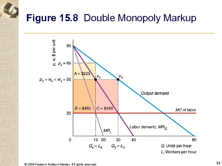 Figure 15. 8 Double Monopoly Markup © 2009 Pearson Addison-Wesley. All rights reserved. 31
 Solved Problem 15. 2 § How are consumers affected and how do profits change in the example if the labor monopoly buys the monopoly producer (integrates vertically)? © 2009 Pearson Addison-Wesley. All rights reserved. 32
 Monopsony § A monopsony chooses a price-quantity combination from the industry supply curve that maximizes its profit. © 2009 Pearson Addison-Wesley. All rights reserved. 33
 Monopsony Profit Maximization § Suppose that a firm is the sole employer in town. w marginal expenditure – the additional cost of hiring one more worker depends on the shape of the supply curve. © 2009 Pearson Addison-Wesley. All rights reserved. 34
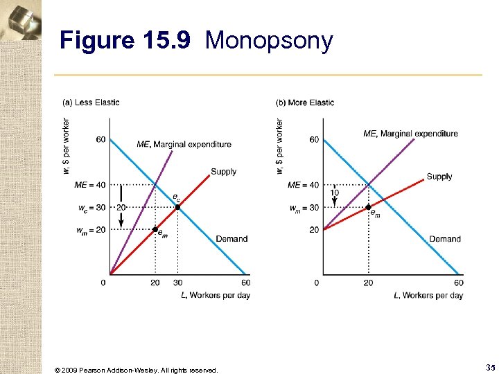 Figure 15. 9 Monopsony © 2009 Pearson Addison-Wesley. All rights reserved. 35
 Monopsony Profit Maximization (cont). § Any buyer buys labor services up to the point at which the marginal value of the last unit of a factor equals the firm’s marginal expenditure. § Monopsony power - the ability of a single buyer to pay less than the competitive price profitably. © 2009 Pearson Addison-Wesley. All rights reserved. 36
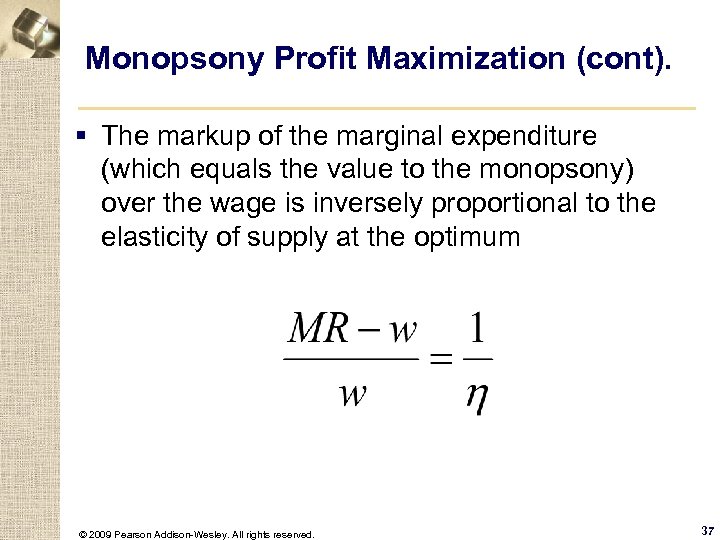 Monopsony Profit Maximization (cont). § The markup of the marginal expenditure (which equals the value to the monopsony) over the wage is inversely proportional to the elasticity of supply at the optimum © 2009 Pearson Addison-Wesley. All rights reserved. 37
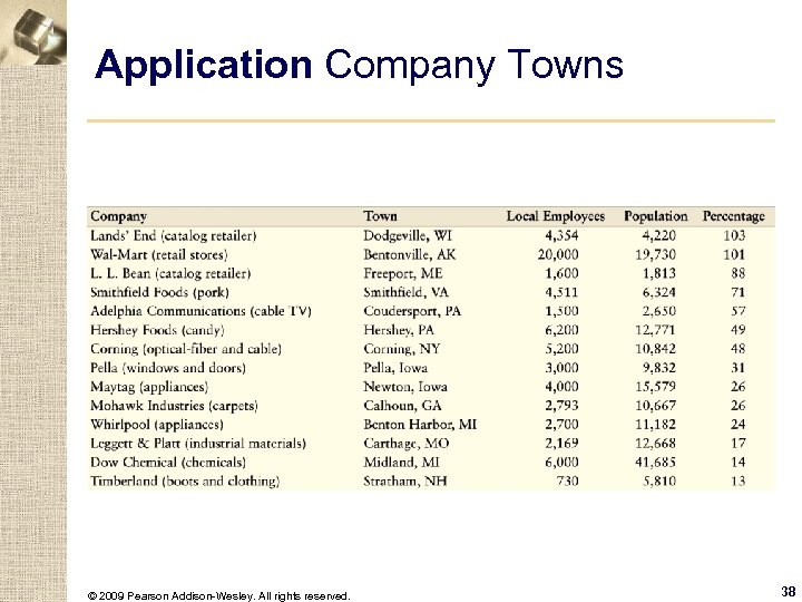 Application Company Towns © 2009 Pearson Addison-Wesley. All rights reserved. 38
 Welfare Effects of Monopsony § By creating a wedge between the value to the monopsony and the value to the suppliers, the monopsony causes a welfare loss in comparison to a competitive market. © 2009 Pearson Addison-Wesley. All rights reserved. 39
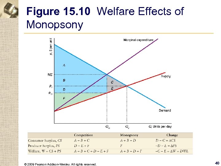 Figure 15. 10 Welfare Effects of Monopsony © 2009 Pearson Addison-Wesley. All rights reserved. 40
 Solved Problem 15. 3 § How does the equilibrium in a labor market with a monopsony employer change if a minimum wage is set at the competitive level? © 2009 Pearson Addison-Wesley. All rights reserved. 41
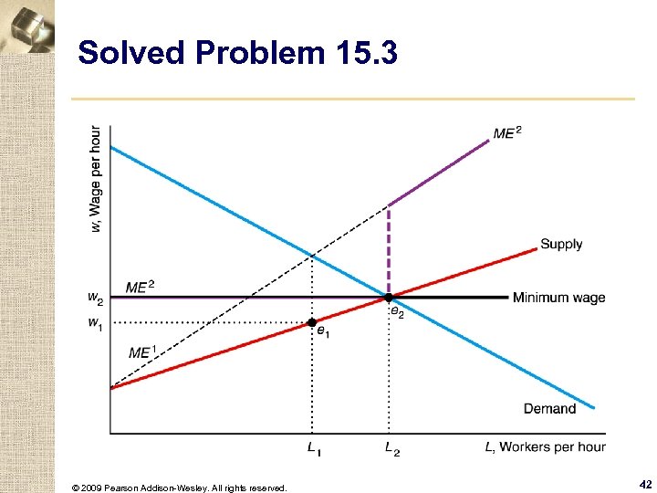 Solved Problem 15. 3 © 2009 Pearson Addison-Wesley. All rights reserved. 42
 Monopsony Price Discrimination § If some consumers have monopsony power while others do not, sellers offer those with monopsony power lower prices. w A monopsony may directly price discriminate in much the same way as a monopoly or an oligopoly. © 2009 Pearson Addison-Wesley. All rights reserved. 43
 Vertical Integration § To sell a good or service to consumers involves many sequential stages of production and sales activities. w Profitability determines how many stages a firm performs itself. © 2009 Pearson Addison-Wesley. All rights reserved. 44
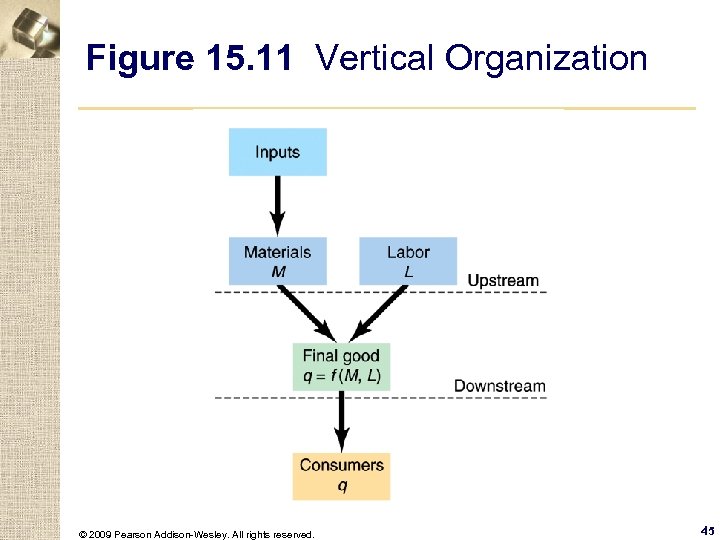 Figure 15. 11 Vertical Organization © 2009 Pearson Addison-Wesley. All rights reserved. 45
 Degree of Vertical Integration § A firm that participates in more than one successive stage of the production or distribution of goods or services is vertically integrated. w A firm may vertically integrate backward and produce its own inputs. © 2009 Pearson Addison-Wesley. All rights reserved. 46
 Degree of Vertical Integration (cont). § Contractual vertical restraints – when a firms control the actions of the firms with whom they deal by writing contracts that restrict the actions of those other firms. w Such tight relationships between firms are referred to as quasi-vertical integration. © 2009 Pearson Addison-Wesley. All rights reserved. 47
 Produce or Buy § Five possible benefits from vertical integration are: w lowering transaction costs, w ensuring a steady supply, w avoiding government intervention, w extending market power to another market, and w eliminating market power. © 2009 Pearson Addison-Wesley. All rights reserved. 48
 Lowering Transaction Costs. § transaction costs - the costs of trading with others besides the price, including the costs of writing and enforcing contracts. § opportunistic behavior - taking advantage of someone when circumstances permit. § asymmetric information - the knowledgeable firm may take advantage of the relatively ignorant firm. © 2009 Pearson Addison-Wesley. All rights reserved. 49
 Ensuring a Steady Supply. § just-in-time - system of having suppliers deliver inputs at the time needed to process them, thus minimizing inventory costs and avoiding bottlenecks. © 2009 Pearson Addison-Wesley. All rights reserved. 50
 Avoiding Government Intervention. § A vertically integrated firm avoids price controls by selling to itself. § Firms also integrate to lower their taxes © 2009 Pearson Addison-Wesley. All rights reserved. 51
 Extending Market Power. § By vertically integrating, a firm may be able to increase its monopoly profits by price discriminating or by monopolizing. © 2009 Pearson Addison-Wesley. All rights reserved. 52


