735af9f69030ff8c72340021b43943e6.ppt
- Количество слайдов: 64
 Chapter Fifteen Factor Markets and Vertical Integration
 Factor Markets and Vertical Integration • In this chapter, we examine four main topics – Competitive factor market – Effect of monopolies on factor markets – Monopsony – Vertical integration © 2007 Pearson Addison-Wesley. All rights reserved. 2
 Competitive Factor Market • Virtually all firms rely on factor markets for at least some inputs. • The firms that buy factors may be competitive price takers or noncompetitive price setters, such as a monopsony. © 2007 Pearson Addison-Wesley. All rights reserved. 3
 Competitive Factor Market • Factor markets are competitive when there are many small buyers and sellers. • Our earlier analysis of the competitive supply curve applies to factor markets. © 2007 Pearson Addison-Wesley. All rights reserved. 4
 Short-Run Factor Demand of a Firm • A profit-maximizing firm’s demand for a factor of production is downward sloping: The higher the price of an input, the less the firm wants to buy. • In the short, a firm has a fixed amount of capital, , and can vary the number of workers, , it employs. © 2007 Pearson Addison-Wesley. All rights reserved. 5
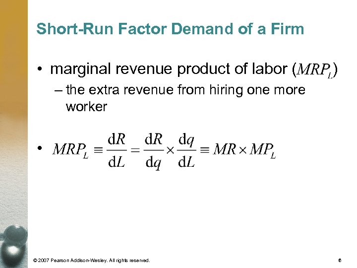 Short-Run Factor Demand of a Firm • marginal revenue product of labor ( ) – the extra revenue from hiring one more worker • © 2007 Pearson Addison-Wesley. All rights reserved. 6
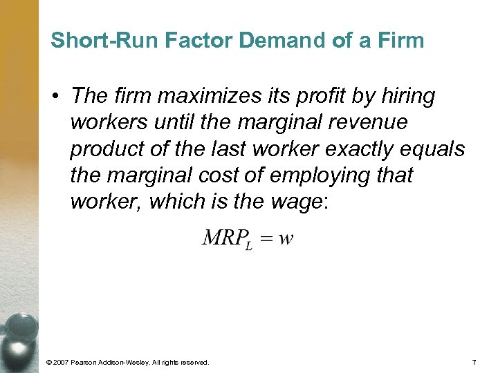 Short-Run Factor Demand of a Firm • The firm maximizes its profit by hiring workers until the marginal revenue product of the last worker exactly equals the marginal cost of employing that worker, which is the wage: © 2007 Pearson Addison-Wesley. All rights reserved. 7
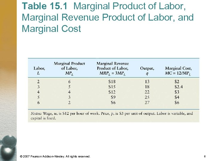 Table 15. 1 Marginal Product of Labor, Marginal Revenue Product of Labor, and Marginal Cost © 2007 Pearson Addison-Wesley. All rights reserved. 8
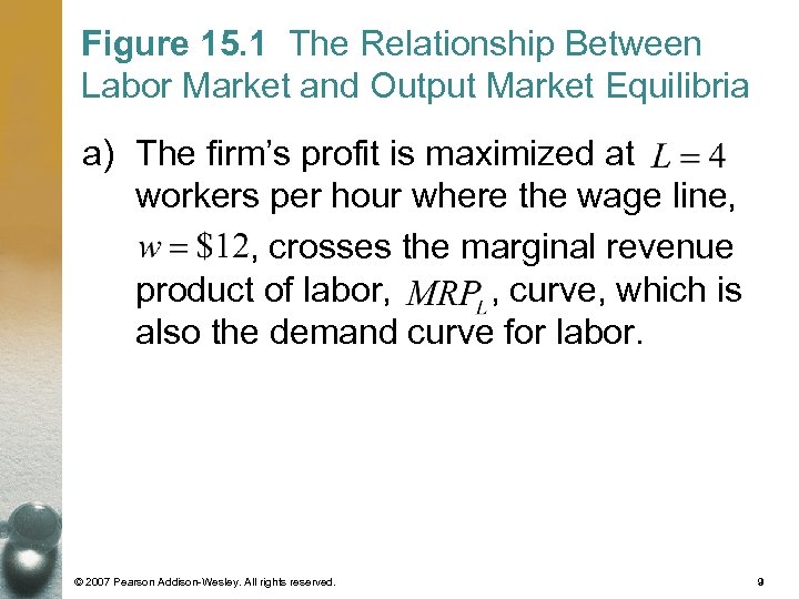 Figure 15. 1 The Relationship Between Labor Market and Output Market Equilibria a) The firm’s profit is maximized at workers per hour where the wage line, , crosses the marginal revenue product of labor, , curve, which is also the demand curve for labor. © 2007 Pearson Addison-Wesley. All rights reserved. 9
 Figure 15. 1 The Relationship Between Labor Market and Output Market Equilibria b) The firm’s profit is maximized at 22 units of output (produced by 4 workers), for which its marginal cost, , curve equals the market price, . © 2007 Pearson Addison-Wesley. All rights reserved. 10
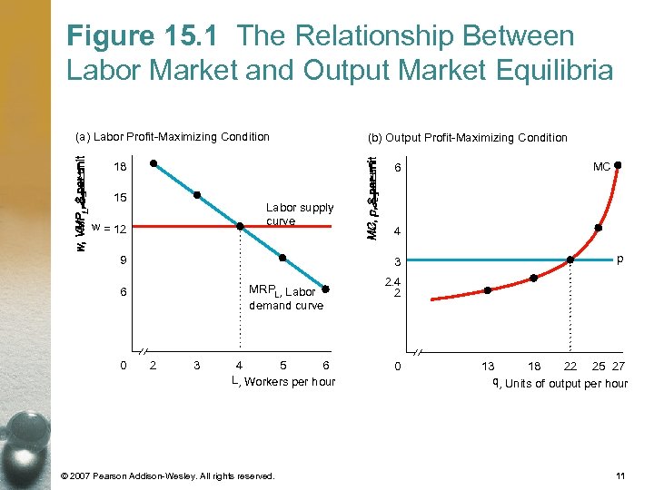 Figure 15. 1 The Relationship Between Labor Market and Output Market Equilibria (a) Labor Profit-Maximizing Condition 18 6 15 Labor supply curve w = 12 9 MRPL, Labor demand curve 2 3 4 5 6 L, Workers per hour © 2007 Pearson Addison-Wesley. All rights reserved. MC 4 3 6 0 (b) Output Profit-Maximizing Condition p 2. 4 2 0 13 18 22 25 27 q, Units of output per hour 11
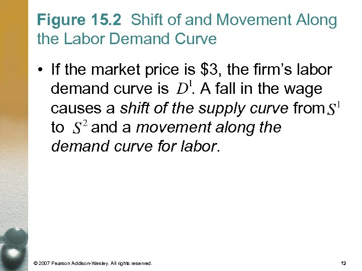 Figure 15. 2 Shift of and Movement Along the Labor Demand Curve • If the market price is $3, the firm’s labor demand curve is. A fall in the wage causes a shift of the supply curve from to and a movement along the demand curve for labor. © 2007 Pearson Addison-Wesley. All rights reserved. 12
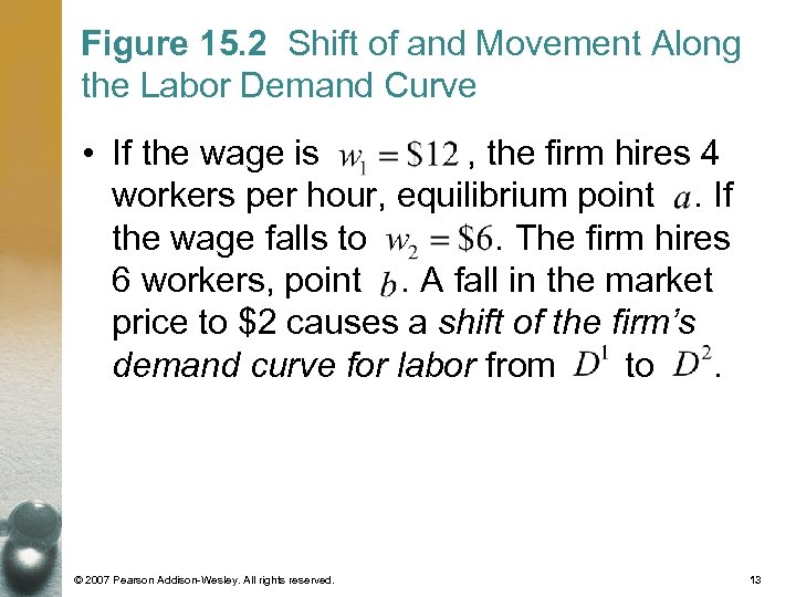 Figure 15. 2 Shift of and Movement Along the Labor Demand Curve • If the wage is , the firm hires 4 workers per hour, equilibrium point. If the wage falls to. The firm hires 6 workers, point. A fall in the market price to $2 causes a shift of the firm’s demand curve for labor from to. © 2007 Pearson Addison-Wesley. All rights reserved. 13
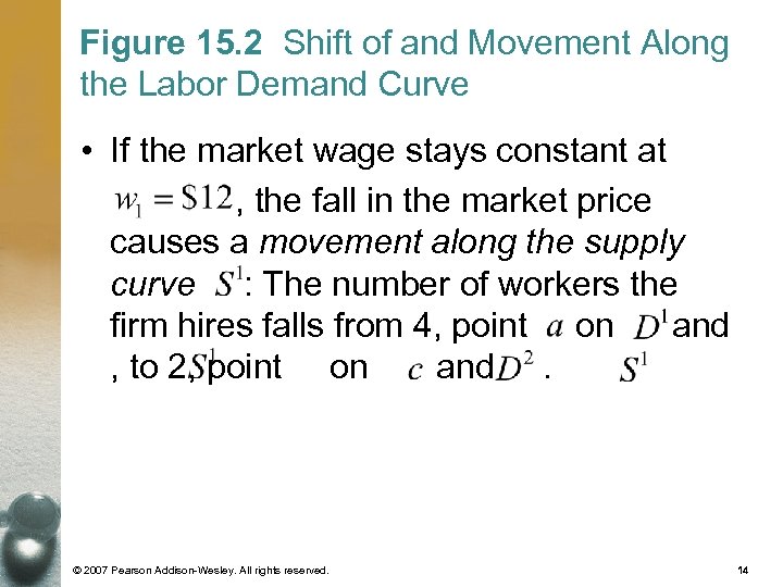 Figure 15. 2 Shift of and Movement Along the Labor Demand Curve • If the market wage stays constant at , the fall in the market price causes a movement along the supply curve : The number of workers the firm hires falls from 4, point on and , to 2, point on and. © 2007 Pearson Addison-Wesley. All rights reserved. 14
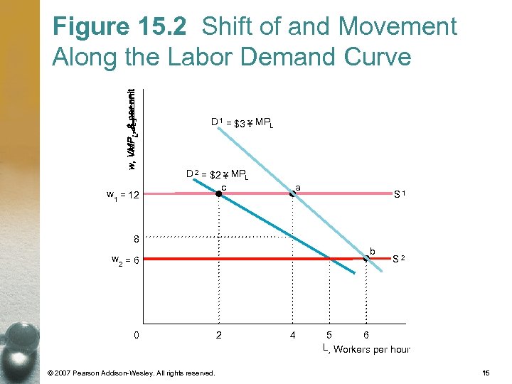 Figure 15. 2 Shift of and Movement Along the Labor Demand Curve D 1 = $3 ¥ MPL w = 12 1 D 2 = $2 ¥ MPL c a S 1 8 b w 2 = 6 0 © 2007 Pearson Addison-Wesley. All rights reserved. 2 4 S 2 5 6 L, Workers per hour 15
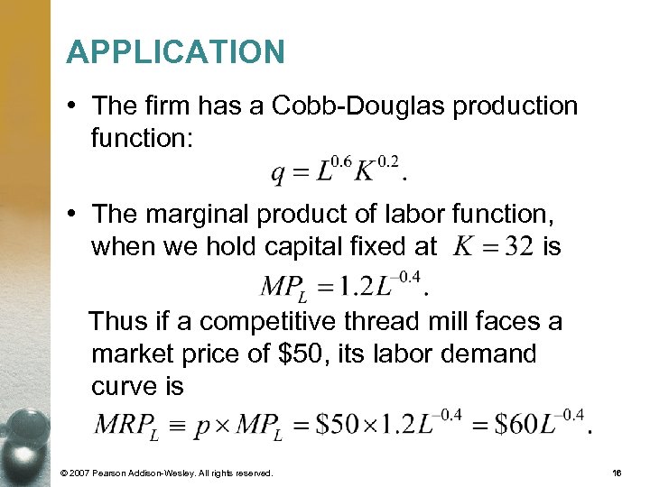 APPLICATION • The firm has a Cobb-Douglas production function: • The marginal product of labor function, when we hold capital fixed at is Thus if a competitive thread mill faces a market price of $50, its labor demand curve is © 2007 Pearson Addison-Wesley. All rights reserved. 16
 Long-Run Factor Demand • In the long run, the firm may vary all of its putout. Now if the wage of labor rises, the firm adjusts both labor and capital. The long-run labor demand curve takes account of changes in the firm’s use of capital as the wage rises. © 2007 Pearson Addison-Wesley. All rights reserved. 17
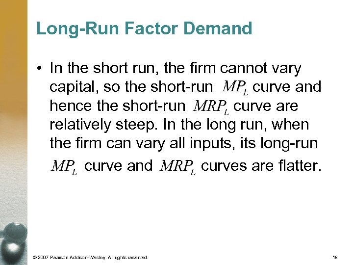 Long-Run Factor Demand • In the short run, the firm cannot vary capital, so the short-run curve and hence the short-run curve are relatively steep. In the long run, when the firm can vary all inputs, its long-run curve and curves are flatter. © 2007 Pearson Addison-Wesley. All rights reserved. 18
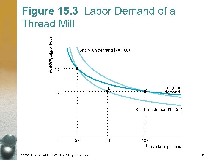 Figure 15. 3 Labor Demand of a Thread Mill K Short-run demand ( = 108) 15 a b 10 c Long-run demand Short-run demand. K = 32) ( 0 32 © 2007 Pearson Addison-Wesley. All rights reserved. 88 162 L, Workers per hour 19
 Factor Market Demand • A factor market demand curve is the sum of the factor demand curves of the various firms that use the input. Determining a factor market demand curve is more difficult than deriving consumer’s market demand for a final good. © 2007 Pearson Addison-Wesley. All rights reserved. 20
 Factor Market Demand • To derive the labor market demand curve, we first determine the labor demand curve for each output market and then sum across output markets to obtain the factor market demand curve. © 2007 Pearson Addison-Wesley. All rights reserved. 21
 The Marginal Revenue Product Approach • Earlier we derived the factor demand of a competitive firm that took the output market price as given. The problem we face is that the output market price depends on the factor’s price. © 2007 Pearson Addison-Wesley. All rights reserved. 22
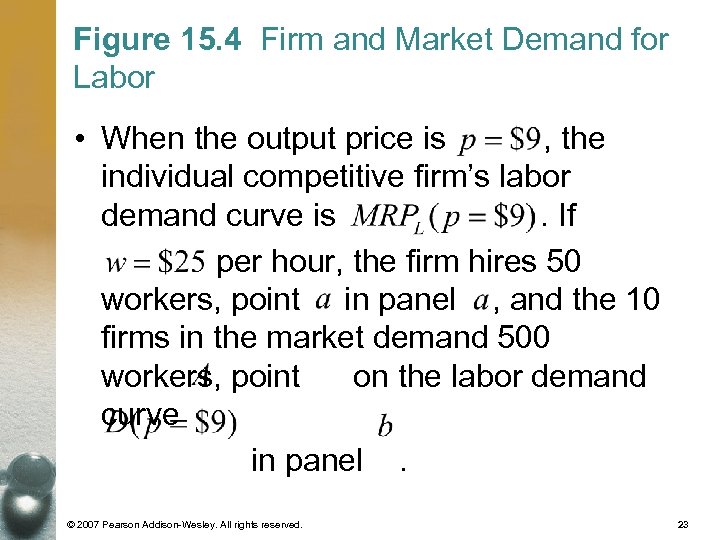 Figure 15. 4 Firm and Market Demand for Labor • When the output price is , the individual competitive firm’s labor demand curve is. If per hour, the firm hires 50 workers, point in panel , and the 10 firms in the market demand 500 workers, point on the labor demand curve in panel. © 2007 Pearson Addison-Wesley. All rights reserved. 23
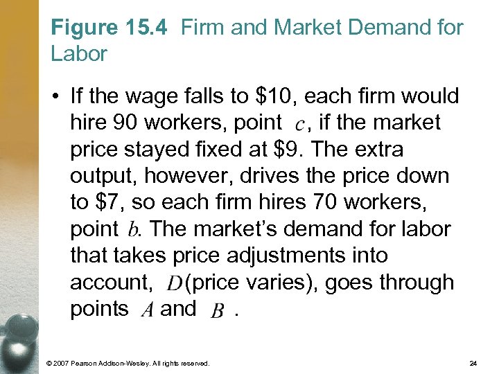 Figure 15. 4 Firm and Market Demand for Labor • If the wage falls to $10, each firm would hire 90 workers, point , if the market price stayed fixed at $9. The extra output, however, drives the price down to $7, so each firm hires 70 workers, point. The market’s demand for labor that takes price adjustments into account, (price varies), goes through points and. © 2007 Pearson Addison-Wesley. All rights reserved. 24
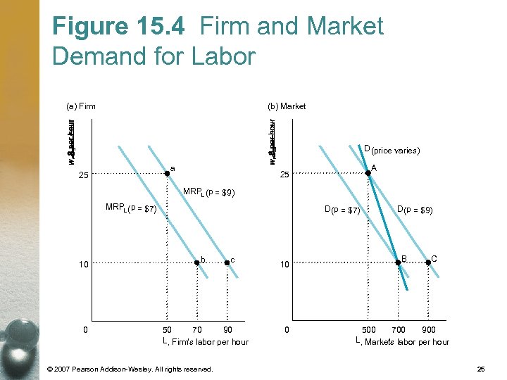 Figure 15. 4 Firm and Market Demand for Labor (b) Market (a) Firm D (price varies) a 25 A 25 MRPL ( p = $9) MRPL ( p = $7) 10 0 D (p = $7) b c 50 70 90 L, Firm’s labor per hour © 2007 Pearson Addison-Wesley. All rights reserved. 10 0 D (p = $9) B C 500 700 900 L, Markets labor per hour ’ 25
 An Alternative Approach • It takes one microchip, which costs , and one plastic case, which costs , to produce a calculator, so the marginal cost of a calculator is. Competitive firms operate where the price of a calculator is. Thus the demand curve for a microchip lies below that of a calculator. © 2007 Pearson Addison-Wesley. All rights reserved. 26
 Figure 15. 5 Demand for Microchips in Calculators pp Demand for calculators Demand for microchips Q, Calculators per day M, Microchips per day © 2007 Pearson Addison-Wesley. All rights reserved. 27
 Competitive Factor Market Equilibrium • The intersection of the factor market demand curve and the factor market supply curve determines the competitive factor market equilibrium. © 2007 Pearson Addison-Wesley. All rights reserved. 28
 Competitive Factor Market Equilibrium • Factor prices are equalized across markets. For example, if wages were higher in one industry than in another, workers would shift from the low-wage industry to the high-wage industry until the wages were equalized. © 2007 Pearson Addison-Wesley. All rights reserved. 29
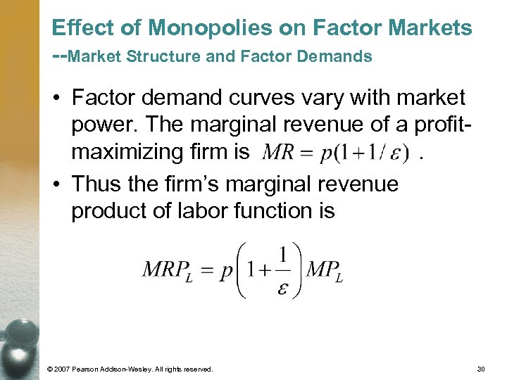 Effect of Monopolies on Factor Markets --Market Structure and Factor Demands • Factor demand curves vary with market power. The marginal revenue of a profitmaximizing firm is. • Thus the firm’s marginal revenue product of labor function is © 2007 Pearson Addison-Wesley. All rights reserved. 30
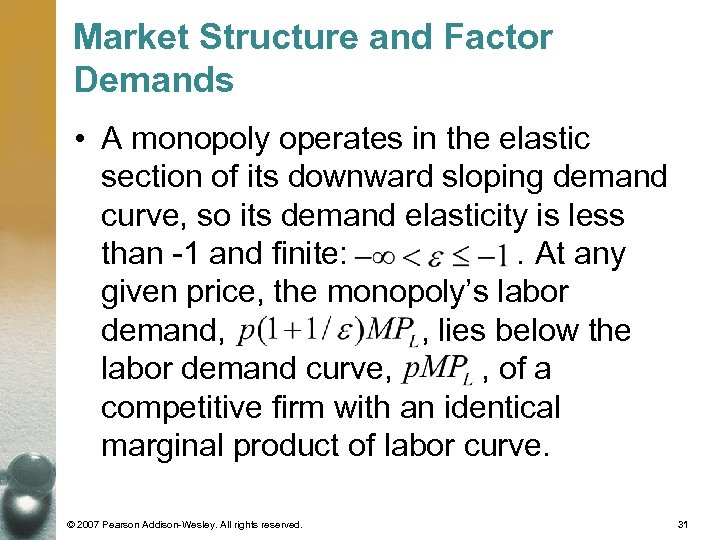 Market Structure and Factor Demands • A monopoly operates in the elastic section of its downward sloping demand curve, so its demand elasticity is less than -1 and finite: . At any given price, the monopoly’s labor demand, , lies below the labor demand curve, , of a competitive firm with an identical marginal product of labor curve. © 2007 Pearson Addison-Wesley. All rights reserved. 31
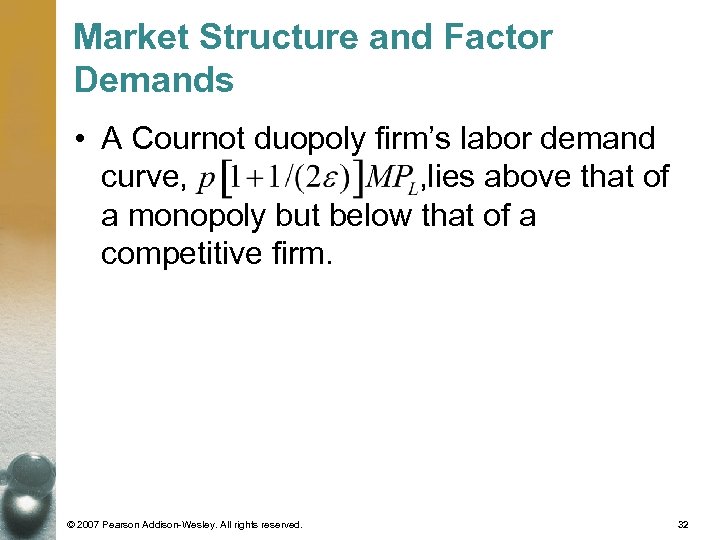 Market Structure and Factor Demands • A Cournot duopoly firm’s labor demand curve, , lies above that of a monopoly but below that of a competitive firm. © 2007 Pearson Addison-Wesley. All rights reserved. 32
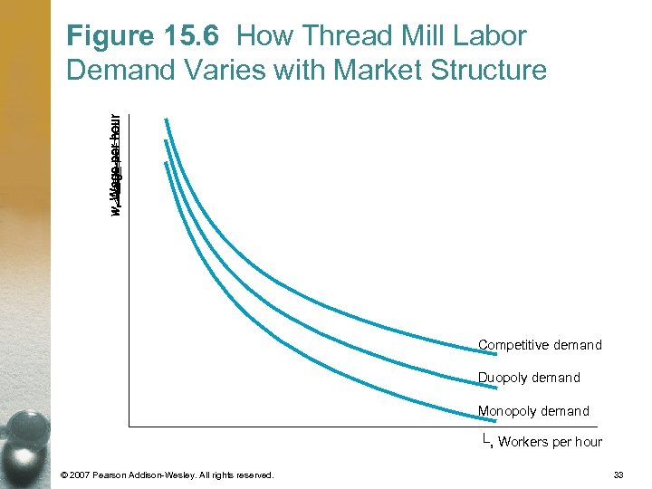 Figure 15. 6 How Thread Mill Labor Demand Varies with Market Structure Competitive demand Duopoly demand Monopoly demand L, Workers per hour © 2007 Pearson Addison-Wesley. All rights reserved. 33
 A Model of Market Power in Input and Output Markets • When a firm with market power in either the factor or the output market raises its price, the price to final consumers rises. As a result, consumers buy fewer units, so fewer units of the input are demanded. © 2007 Pearson Addison-Wesley. All rights reserved. 34
 Competitive Factor and Output Markets • The labor demand function is the same as the output demand function, where we replace with and with : • The intersection of this output supply curve and the output demand curve occurs at and. A competitive firm’s average cost, , exactly equals the price at which it sells its good, , so the competitive firm breaks even. © 2007 Pearson Addison-Wesley. All rights reserved. 35
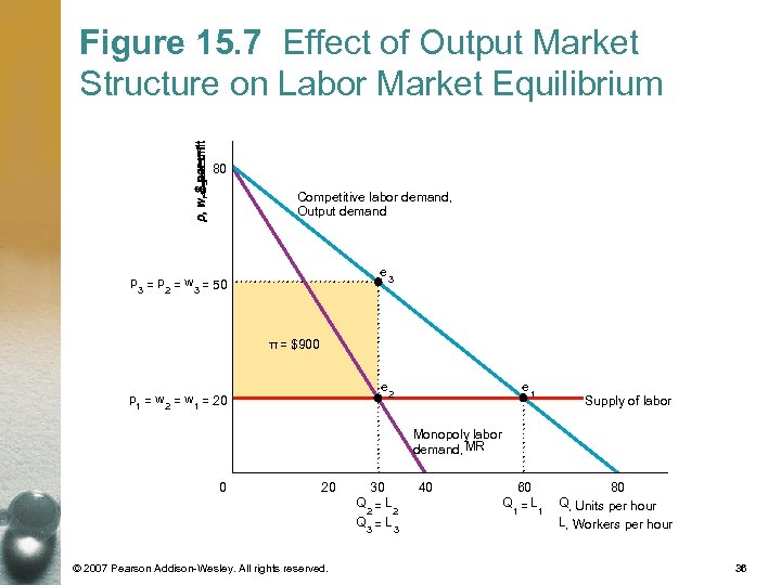 Figure 15. 7 Effect of Output Market Structure on Labor Market Equilibrium 80 Competitive labor demand, Output demand e 3 p = w = 50 3 2 3 π = $900 e 2 p = w = 20 1 2 1 e 1 Supply of labor Monopoly labor demand, MR 0 20 30 Q =L 2 2 Q =L 3 © 2007 Pearson Addison-Wesley. All rights reserved. 3 40 60 Q =L 1 1 80 Q, Units per hour L, Workers per hour 36
 Competitive Factor Market and Monoplized Output Market • Because the monopoly’s marginal product of labor is 1, its demand curve for labor equals its marginal revenue curve: © 2007 Pearson Addison-Wesley. All rights reserved. 37
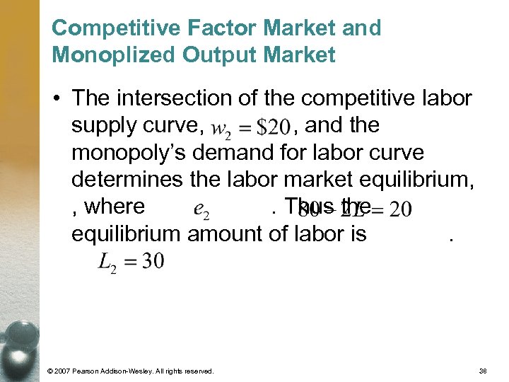 Competitive Factor Market and Monoplized Output Market • The intersection of the competitive labor supply curve, , and the monopoly’s demand for labor curve determines the labor market equilibrium, , where. Thus the equilibrium amount of labor is. © 2007 Pearson Addison-Wesley. All rights reserved. 38
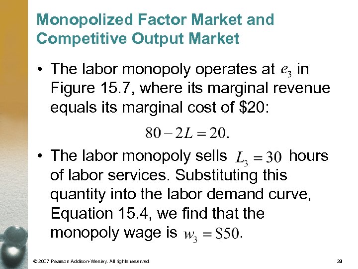 Monopolized Factor Market and Competitive Output Market • The labor monopoly operates at in Figure 15. 7, where its marginal revenue equals its marginal cost of $20: • The labor monopoly sells hours of labor services. Substituting this quantity into the labor demand curve, Equation 15. 4, we find that the monopoly wage is. © 2007 Pearson Addison-Wesley. All rights reserved. 39
 Monopolized Factor Market and Competitive Output Market • The profit goes to the monopoly regardless of which market is monopolized. © 2007 Pearson Addison-Wesley. All rights reserved. 40
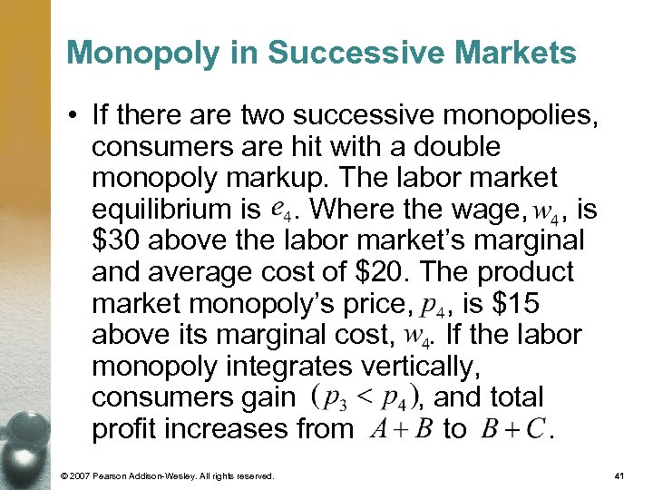 Monopoly in Successive Markets • If there are two successive monopolies, consumers are hit with a double monopoly markup. The labor market equilibrium is. Where the wage, , is $30 above the labor market’s marginal and average cost of $20. The product market monopoly’s price, , is $15 above its marginal cost, . If the labor monopoly integrates vertically, consumers gain , and total profit increases from to. © 2007 Pearson Addison-Wesley. All rights reserved. 41
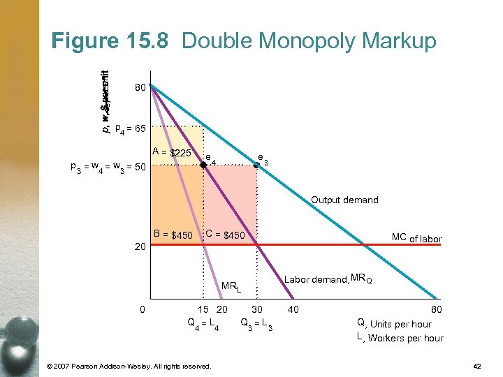 Figure 15. 8 Double Monopoly Markup 80 p = 65 4 A = $225 p = w = 50 3 4 3 e e 4 3 Output demand B = $450 C = $450 MC of labor 20 MRL 0 15 20 Q =L 4 4 © 2007 Pearson Addison-Wesley. All rights reserved. 30 Q =L 3 3 Labor demand, MRQ 40 80 Q, Units per hour L, Workers per hour 42
 Monopsony • A monopsony, a single buyer in a market, chooses a price-quantity combination from the industry supply curve that maximizes its profit. • A monopsony is the mirror image of monopoly, and it exercises its market power by buying at a price below the price that competitive buyers would pay. © 2007 Pearson Addison-Wesley. All rights reserved. 43
 Monopsony Profit Maximization a) The marginal expenditure curve—the monopsony’s marginal cost of buying one more unit—lies above the upwardsloping market supply curve. The monopsony equilibrium, , occurs where the marginal expenditure curve intersects the monopsony’s demand curve. The monopsony buys fewer units at a lower price, , than a competitive market, , would. © 2007 Pearson Addison-Wesley. All rights reserved. 44
 Monopsony Profit Maximization b) The supply curve is more elastic at the optimum than in (a), so the value that the monopsony places on the last unit (which equals the marginal expenditure of $40) exceeds the price the monopsony pays, , by less in (a). © 2007 Pearson Addison-Wesley. All rights reserved. 45
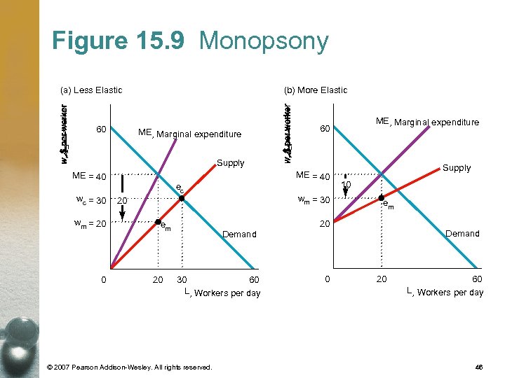 Figure 15. 9 Monopsony (b) More Elastic (a) Less Elastic 60 ME, Marginal expenditure 60 Supply ME = 40 wc = 30 wm = 20 0 ec wm = 30 20 em 20 Demand 30 60 L, Workers per day © 2007 Pearson Addison-Wesley. All rights reserved. Supply 10 em 20 0 Demand 20 60 L, Workers per day 46
 Monopsony Profit Maximization • Monopsony power is the ability of a single buyer to pay less than the competitive price profitable. The size if the gap between the value the monopsony places on the last worker (the height of its demand curve) and the wage it pays (the height of the supply curve) depends on the elasticity of supply at the monopsony optimum. © 2007 Pearson Addison-Wesley. All rights reserved. 47
 Welfare Effects of Monopsony • By setting a price, , below the competitive level, , a monopsony causes too little to be sold by the supplying market, thereby reducing welfare. © 2007 Pearson Addison-Wesley. All rights reserved. 48
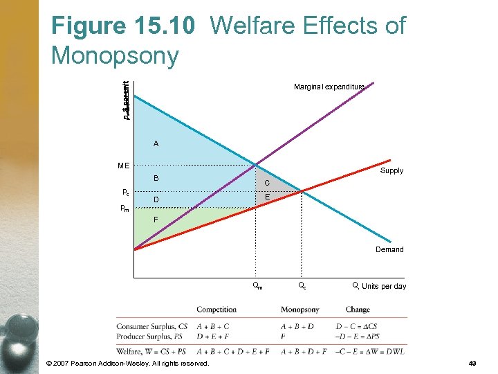 Figure 15. 10 Welfare Effects of Monopsony Marginal expenditure A ME Supply B pc pm C E D F Demand Qm © 2007 Pearson Addison-Wesley. All rights reserved. Qc Q, Units per day 49
 Monopsony Price Discrimination • If some consumers have monopsony power while others do not, sellers offer those with monopsony power lower prices. • A monopsony may directly price discriminate in much the same way as a monopoly or an oligopoly. © 2007 Pearson Addison-Wesley. All rights reserved. 50
 Vertical Integration • To sell a good or service to consumers involves many sequential stages of production and sales activities. Profitability determines how many stages a firm performs itself. © 2007 Pearson Addison-Wesley. All rights reserved. 51
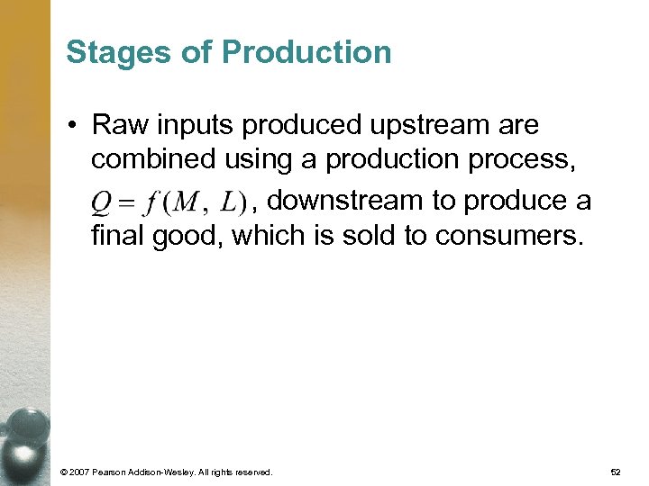 Stages of Production • Raw inputs produced upstream are combined using a production process, , downstream to produce a final good, which is sold to consumers. © 2007 Pearson Addison-Wesley. All rights reserved. 52
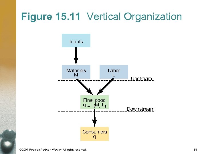 Figure 15. 11 Vertical Organization Inputs Materials M Final good q = f (M, L) Labor L Upstream Downstream Consumers q © 2007 Pearson Addison-Wesley. All rights reserved. 53
 Degree of Vertical Integration • A firm that participates in more than one successive stage of the production or distribution of goods or services is vertically integrated. A firm may vertically integrate backward and produce its own inputs. © 2007 Pearson Addison-Wesley. All rights reserved. 54
 Degree of Vertical Integration • All firms are vertically integrated to some degree, but they differ substantially as to how many successive stages of production they perform internally. It may produce a good but rely on others to market it. Or it may produce some inputs itself and buy others form the market. © 2007 Pearson Addison-Wesley. All rights reserved. 55
 Produce or Buy • Whether a firm vertically integrates, quasi-vertically integrates, or relies on markets depends on which approach is the most profitable. • When deciding whether to integrate vertically, the firm must take into account not only the direct costs of integrating, such as legal fee, but also the higher cost of managing a larger, more complex company. © 2007 Pearson Addison-Wesley. All rights reserved. 56
 Produce or Buy • Five Possible Benefits from Vertical integration – Lowering transaction costs – Ensuring a steady supply – Avoiding government intervention – Extending market power – Eliminating market power © 2007 Pearson Addison-Wesley. All rights reserved. 57
 Lowering Transaction Costs • Probably the most important reason to integrate is to avoid transaction cost: the costs of trading with others besides the price, including the costs of writing and enforcing contracts. © 2007 Pearson Addison-Wesley. All rights reserved. 58
 Lowering Transaction Costs • An important source of transaction costs is opportunistic behavior: taking advantage of someone when circumstances permit. © 2007 Pearson Addison-Wesley. All rights reserved. 59
 Ensuring a Steady Supply • Like the electronic game manufacturer, many firms are at mercy of their suppliers. A supplier that delivers a crucial part late imposes substantial costs on these manufactures. © 2007 Pearson Addison-Wesley. All rights reserved. 60
 Avoiding Government Intervention • Firms may also vertically integrate to avoid government price control, taxes, and regulations. A vertically integrated firm avoids price controls by selling to itself. © 2007 Pearson Addison-Wesley. All rights reserved. 61
 Avoiding Government Intervention • Firms also integrate to lower their taxes. By shifting profits from a high-tax jurisdiction to a low-tax jurisdiction, a firm can increase its after-tax profits. • Government regulations create additional incentives for a firm to integrate vertically (or horizontally) when the profits of only one division of a firm are regulated. © 2007 Pearson Addison-Wesley. All rights reserved. 62
 Extending Market Power • By vertically integrating, a firm may be able to increase its monopoly profits by price discriminating or by monopolizing. © 2007 Pearson Addison-Wesley. All rights reserved. 63
 Eliminating Market Power • A firm that faces a monopsony buyer or monopoly seller may try to eliminate that market power by vertically integrating. © 2007 Pearson Addison-Wesley. All rights reserved. 64


