Chapter 9 The Analysis of Competitive Markets

Chapter 9 The Analysis of Competitive Markets

Consumer and Producer Surplus l When government controls price, some people are better off m May be able to buy a good at a lower price l But what is the effect on society as a whole? m Is total welfare higher or lower and by how much? l A way to measure gains and losses from government policies is needed © 2005 Pearson Education, Inc. Chapter 9 2

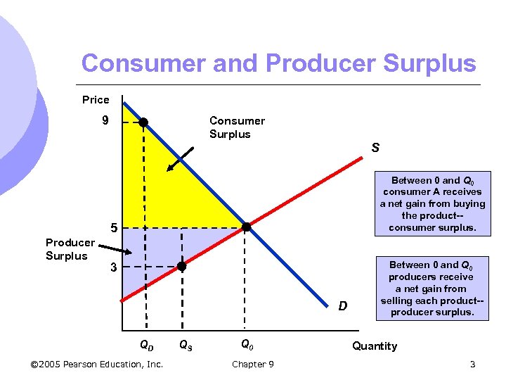Consumer and Producer Surplus Price 9 Consumer Surplus S Between 0 and Q 0 consumer A receives a net gain from buying the product-consumer surplus. 5 Producer Surplus 3 D QD © 2005 Pearson Education, Inc. QS Q 0 Chapter 9 Between 0 and Q 0 producers receive a net gain from selling each product-producer surplus. Quantity 3

Consumer and Producer Surplus l To determine the welfare effect of a governmental policy, we can measure the gain or loss in consumer and producer surplus l Welfare Effects m Gains and losses to producers and consumers © 2005 Pearson Education, Inc. Chapter 9 4

Consumer and Producer Surplus l When price is held too low, the quantity demanded increases and quantity supplied decreases l Some consumers are worse off because they can no longer buy the good m Decrease in consumer surplus l Some consumers are better off because they can buy it at a lower price m Increase © 2005 Pearson Education, Inc. in consumer surplus Chapter 9 5

Consumer and Producer Surplus l Producers sell less at a lower price l Some producers are no longer in the market l Both of these producer groups lose and producer surplus decreases l The economy as a whole is worse off since surplus that used to belong to producers or consumers is simply gone © 2005 Pearson Education, Inc. Chapter 9 6

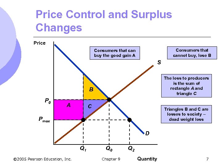Price Control and Surplus Changes Price Consumers that cannot buy, lose B Consumers that can buy the good gain A S The loss to producers is the sum of rectangle A and triangle C B P 0 A C Triangles B and C are losses to society – dead weight loss Pmax D Q 1 © 2005 Pearson Education, Inc. Q 0 Chapter 9 Q 2 Quantity 7

Price Controls and Welfare Effects l The total loss is equal to area B + C l The deadweight loss is the inefficiency of the price controls – the total loss in surplus (consumer plus producer) l If demand is sufficiently inelastic, losses to consumers may be fairly large m This can have effects in political decisions © 2005 Pearson Education, Inc. Chapter 9 8

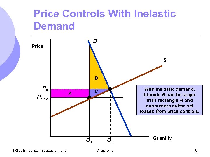Price Controls With Inelastic Demand D Price S B P 0 Pmax A Q 1 © 2005 Pearson Education, Inc. With inelastic demand, triangle B can be larger than rectangle A and consumers suffer net losses from price controls. C Q 2 Chapter 9 Quantity 9

The Efficiency of a Competitive Market l In the evaluation of markets, we often talk about whether it reaches economic efficiency m Maximization of aggregate consumer and producer surplus l Policies such as price controls that cause dead weight losses in society are said to impose an efficiency cost on the economy © 2005 Pearson Education, Inc. Chapter 9 10

The Efficiency of a Competitive Market l If efficiency is the goal, then you can argue that leaving markets alone is the answer l However, sometimes market failures occur m Prices fail to provide proper signals to consumers and producers m Leads to inefficient unregulated competitive market © 2005 Pearson Education, Inc. Chapter 9 11

Types of Market Failures 1. Externalities m m Costs or benefits that are not reflected in market supply and demand (e. g. pollution) Costs or benefits are experienced by a third party not involved in transaction 2. Lack of Information m Imperfect information prevents consumers from making utility-maximizing decisions l Government intervention may be desirable in these cases © 2005 Pearson Education, Inc. Chapter 9 12

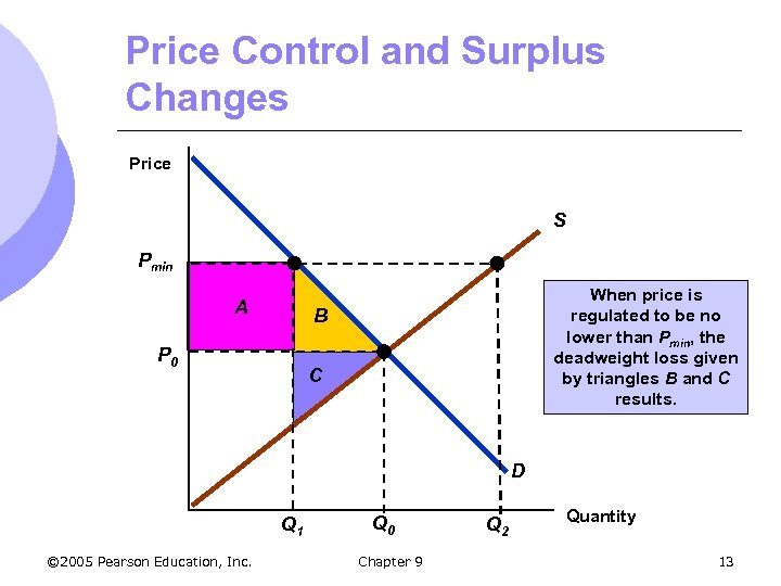Price Control and Surplus Changes Price S Pmin A When price is regulated to be no lower than Pmin, the deadweight loss given by triangles B and C results. B P 0 C D Q 1 © 2005 Pearson Education, Inc. Q 0 Chapter 9 Q 2 Quantity 13

The Market for Human Kidneys l The 1984 National Organ Transplantation Act prohibits the sale of organs for transplantation l What has been the impact of the Act? l We can measure this using the supply and demand for kidneys from estimated data m Supply: QS = 8, 000 + 0. 2 P m Demand: QD = 16, 000 - 0. 2 P © 2005 Pearson Education, Inc. Chapter 9 14

The Market for Human Kidneys l Since the sale of organs is not allowed, the amount available depends on the amount donated m Supply of donated kidneys is limited to 8, 000 l The welfare effect of this supply constraint can be analyzed using consumer and producer surplus in the kidney market © 2005 Pearson Education, Inc. Chapter 9 15

The Market for Human Kidneys l Suppliers: m Those who supply them are not paid the market price, estimated at $20, 000 l Loss of surplus equal to area A = $160 million m Some who would donate for the equilibrium price do not donate in the current market l Loss m Total © 2005 Pearson Education, Inc. of surplus equal to area C = $40 million ‘producer’ loss of A + C = $200 million Chapter 9 16

The Market for Human Kidneys l Recipients: m Since they do not have to pay for the kidney, they gain rectangle A ($160 million) since price is $0 m Those who cannot obtain a kidney lose surplus equal to triangle B ($40 million) m Net increase in surplus of recipients of $160 $40 = $120 million l Dead Weight Loss of C + B = $80 million © 2005 Pearson Education, Inc. Chapter 9 17

The Market for Human Kidneys l Other Inefficiency Costs m Allocation is not necessarily to those who value the kidneys the most m Price may increase to $40, 000, the equilibrium price, with hospitals getting the price © 2005 Pearson Education, Inc. Chapter 9 18

The Market for Kidneys S’ Price The loss to suppliers is seen in areas A & C. $40, 000 D $30, 000 If kidneys are zero cost, consumer gain would be A minus B. B $20, 000 A and D measure the total value of kidneys when supply is constrained. C A $10, 000 0 4, 000 © 2005 Pearson Education, Inc. S D 8, 000 Chapter 9 12, 000 Quantity 19

The Market for Human Kidneys l Arguments in favor of prohibiting the sale of organs: 1. 2. Imperfect information about donor’s health and screening Unfair to allocate according to the ability to pay Holding price below equilibrium will create shortages l Organs versus artificial substitutes l © 2005 Pearson Education, Inc. Chapter 9 20

Minimum Prices l Periodically, government policy seeks to raise prices above market-clearing levels m Minimum wage law m Regulation of airlines m Agricultural policies l We will investigate this by looking at the minimum wage legislation © 2005 Pearson Education, Inc. Chapter 9 21

Minimum Prices Price S Pmin A D measures total cost of increased production not sold. B C P 0 If producers produce Q 2, the amount Q 2 - Q 3 will go unsold. The change in producer surplus will be A - C - D. Producers may be worse off. D D Q 3 © 2005 Pearson Education, Inc. Q 0 Chapter 9 Q 2 Quantity 22

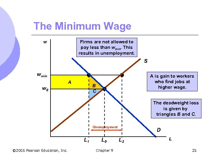The Minimum Wage Firms are not allowed to pay less than wmin. This results in unemployment. w S wmin A A is gain to workers who find jobs at higher wage. B C w 0 The deadweight loss is given by triangles B and C. Unemployment L 1 © 2005 Pearson Education, Inc. L 0 Chapter 9 D L 23

Price Supports l Much of agricultural policy is based on a system of price supports m Prices set by government above free-market level and maintained by governmental purchases of excess supply © 2005 Pearson Education, Inc. Chapter 9 24

Price Supports l What are the impacts on consumers, producers and the federal budget? l Consumers m Quantity demanded falls and quantity supplied increases m Government buys surplus m Consumers must pay higher price for the good m Loss in consumer surplus equal to A+B © 2005 Pearson Education, Inc. Chapter 9 25

Price Supports l Producers m Gain since they are selling more at a higher price m Producer surplus increases by A+B+D l Government m Cost of buying the surplus, which is funded by taxes, so indirect cost on consumers m Cost to government = (Q 2 -Q 1)PS © 2005 Pearson Education, Inc. Chapter 9 26

Price Supports l Government may be able to “dump” some of the goods in the foreign markets m Hurts domestic producers that government is trying to help in the first place l Total welfare effect of policy CS + PS – Govt. cost = D – (Q 2 -Q 1)PS l Society is worse off overall l Less costly to simply give farmers the money © 2005 Pearson Education, Inc. Chapter 9 27

Price Supports Price S Qg Ps A P 0 To maintain a price Ps the government buys quantity Qg. D B Net Loss to society is E + B. D + Qg E D Q 1 © 2005 Pearson Education, Inc. Q 0 Q 2 Chapter 9 Quantity 28

Production Quotas l The government can also cause the price of a good to rise by reducing supply m Limitations of taxi medallions in New York City m Limitation of required liquor licenses for restaurants © 2005 Pearson Education, Inc. Chapter 9 29

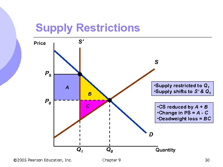Supply Restrictions S’ Price S PS • Supply restricted to Q 1 • Supply shifts to S’ & Q 1 A B P 0 C • CS reduced by A + B • Change in PS = A - C • Deadweight loss = BC D Q 1 © 2005 Pearson Education, Inc. Q 0 Chapter 9 Quantity 30

Import Quotas and Tariffs l Many countries use import quotas and tariffs to keep the domestic price of a product above world levels m Import quotas: Limit on the quantity of a good that can be imported m Tariff: Tax on an imported good l This allows domestic producers to enjoy higher profits l Cost to consumers is high © 2005 Pearson Education, Inc. Chapter 9 31

Import Quotas and Tariffs l With lower world price, domestic consumers have incentive to purchase from abroad m Domestic price falls to world price and imports equal difference between quantity supplied and quantity demanded l Domestic industry might convince government to protect industry by eliminating imports m Quota © 2005 Pearson Education, Inc. of zero or high tariff Chapter 9 32

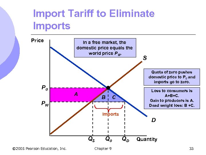Import Tariff to Eliminate Imports Price P 0 In a free market, the domestic price equals the world price PW. S Quota of zero pushes domestic price to P 0 and imports go to zero. A B PW Loss to consumers is A+B+C. Gain to producers is A. Dead weight loss: B +C. C Imports D QS © 2005 Pearson Education, Inc. Q 0 Chapter 9 QD Quantity 33

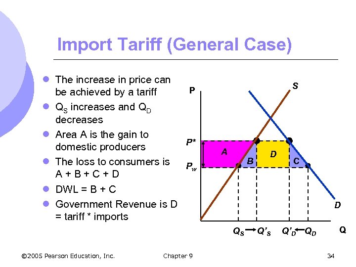Import Tariff (General Case) l The increase in price can P be achieved by a tariff l QS increases and QD decreases l Area A is the gain to P* domestic producers l The loss to consumers is Pw A+B+C+D l DWL = B + C l Government Revenue is D = tariff * imports S A B Chapter 9 C D QS © 2005 Pearson Education, Inc. D Q’S Q’D Q QD 34

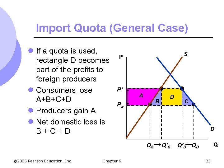Import Quota (General Case) l If a quota is used, rectangle D becomes part of the profits to foreign producers l Consumers lose A+B+C+D l Producers gain A l Net domestic loss is B+C+D S P P* A B Pw Chapter 9 C D QS © 2005 Pearson Education, Inc. D Q’S Q’D Q QD 35

The Sugar Quota Example l The world price of sugar has been as low as 4 cents per pound, while in the U. S. the price has been 20 -25 cents per pound l Sugar quotas have protected the sugar industry but driven up prices l Domestic producers have been better off and so have some foreign producers that have quota rights l Consumers are worse off © 2005 Pearson Education, Inc. Chapter 9 36

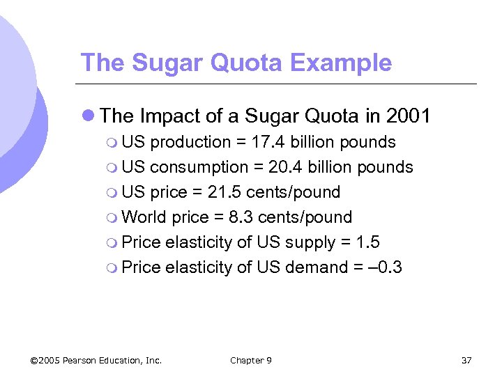The Sugar Quota Example l The Impact of a Sugar Quota in 2001 m US production = 17. 4 billion pounds m US consumption = 20. 4 billion pounds m US price = 21. 5 cents/pound m World price = 8. 3 cents/pound m Price elasticity of US supply = 1. 5 m Price elasticity of US demand = – 0. 3 © 2005 Pearson Education, Inc. Chapter 9 37

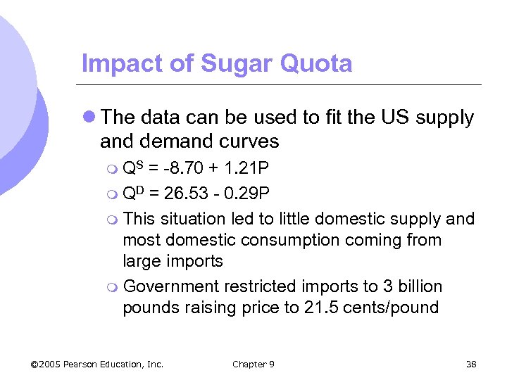Impact of Sugar Quota l The data can be used to fit the US supply and demand curves m QS = -8. 70 + 1. 21 P m QD = 26. 53 - 0. 29 P m This situation led to little domestic supply and most domestic consumption coming from large imports m Government restricted imports to 3 billion pounds raising price to 21. 5 cents/pound © 2005 Pearson Education, Inc. Chapter 9 38

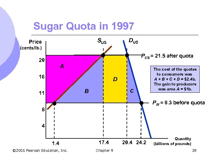Sugar Quota in 1997 DUS SUS Price (cents/lb. ) PUS = 21. 5 after quota 20 A 16 D B 11 C The cost of the quotas to consumers was A + B + C + D = $2. 4 b. The gain to producers was area A = $1 b. PW = 8. 3 before quota 8 4 1. 4 © 2005 Pearson Education, Inc. 17. 4 Chapter 9 20. 4 24. 2 Quantity (billions of pounds) 39

The Impact of a Tax or Subsidy l The government wants to impose a $1. 00 tax on movies. It can do it two ways: m Make the producers pay $1. 00 for each movie ticket they sell m Make consumers pay $1. 00 when they buy each movie l In which option are consumers paying more? © 2005 Pearson Education, Inc. Chapter 9 40

The Impact of a Tax or Subsidy l The burden of a tax (or the benefit of a subsidy) falls partly on the consumer and partly on the producer l How the burden is split between the parties depends on the relative elasticities of demand supply © 2005 Pearson Education, Inc. Chapter 9 41

The Effects of a Specific Tax l For simplicity we will consider a specific tax on a good m Tax of a particular amount per unit sold m Federal and state taxes on gas and cigarettes l For our example, consider a specific tax of $t per widget sold © 2005 Pearson Education, Inc. Chapter 9 42

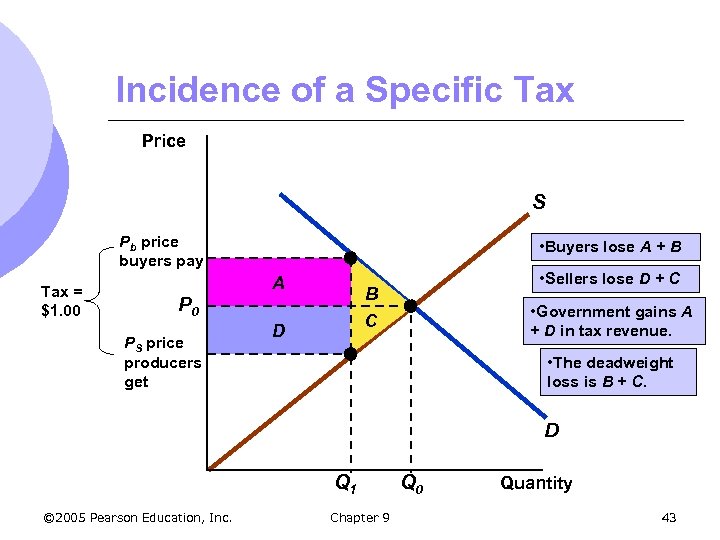Incidence of a Specific Tax Price S Pb price buyers pay Tax = $1. 00 • Buyers lose A + B A B P 0 PS price producers get • Sellers lose D + C • Government gains A + D in tax revenue. C D • The deadweight loss is B + C. D Q 1 © 2005 Pearson Education, Inc. Chapter 9 Q 0 Quantity 43

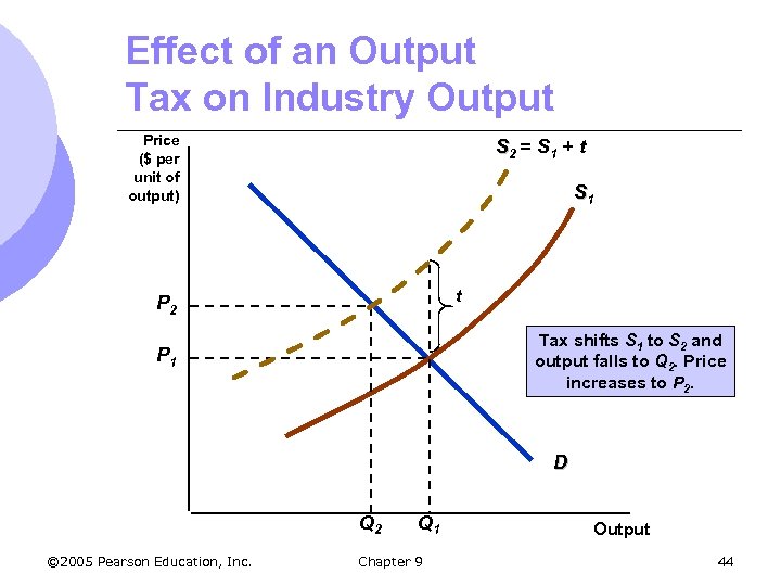Effect of an Output Tax on Industry Output Price ($ per unit of output) S 2 = S 1 + t S 1 t P 2 Tax shifts S 1 to S 2 and output falls to Q 2. Price increases to P 2. P 1 D Q 2 © 2005 Pearson Education, Inc. Q 1 Chapter 9 Output 44

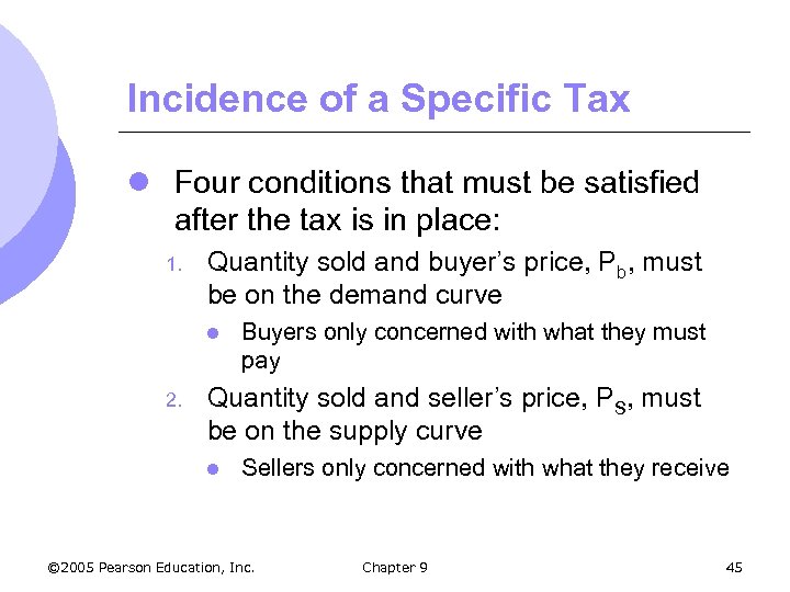Incidence of a Specific Tax l Four conditions that must be satisfied after the tax is in place: 1. Quantity sold and buyer’s price, Pb, must be on the demand curve l 2. Buyers only concerned with what they must pay Quantity sold and seller’s price, PS, must be on the supply curve l Sellers only concerned with what they receive © 2005 Pearson Education, Inc. Chapter 9 45

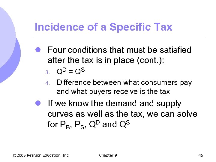Incidence of a Specific Tax l Four conditions that must be satisfied after the tax is in place (cont. ): 3. 4. QD = Q S Difference between what consumers pay and what buyers receive is the tax l If we know the demand supply curves as well as the tax, we can solve for PB, PS, QD and QS © 2005 Pearson Education, Inc. Chapter 9 46

Incidence of a Specific Tax l In the previous example, the tax was shared almost equally by consumers and producers l If demand is relatively inelastic, however, burden of tax will fall mostly on buyers m Cigarettes l If supply is relatively inelastic, the burden of tax will fall mostly on sellers © 2005 Pearson Education, Inc. Chapter 9 47

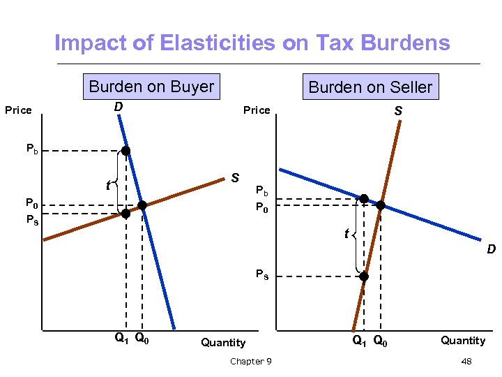Impact of Elasticities on Tax Burdens Burden on Buyer Burden on Seller D Price S Pb S t P 0 PS Pb P 0 t D PS Q 1 Q 0 Quantity Chapter 9 Q 1 Q 0 Quantity 48

The Impact of a Tax or Subsidy l We can calculate the percentage of a tax borne by consumers using pass-through fraction m ES/(ES - E d) m Tells fraction of tax “passed through” to consumers through higher prices m For example, when demand is perfectly inelastic (Ed = 0), the pass-through fraction is 1 – consumers bear 100% of tax © 2005 Pearson Education, Inc. Chapter 9 49

The Effects of a Tax or Subsidy l A subsidy can be analyzed in much the same way as a tax m Payment reducing the buyer’s price below the seller’s price l It can be treated as a negative tax l The seller’s price exceeds the buyer’s price l Quantity increases © 2005 Pearson Education, Inc. Chapter 9 50

Effects of a Subsidy Price S Like a tax, the benefit of a subsidy is split between buyers and sellers, depending upon the elasticities of supply and demand. PS Subsidy P 0 Pb D Q 0 © 2005 Pearson Education, Inc. Chapter 9 Q 1 Quantity 51

Effects of a Subsidy l The benefit of the subsidy accrues mostly to buyers if ED /ES is small l The benefit of the subsidy accrues mostly to sellers if ED /ES is large l As with a tax, using supply and demand curves, and the size of the subsidy, one can solve for resulting prices and quantities © 2005 Pearson Education, Inc. Chapter 9 52

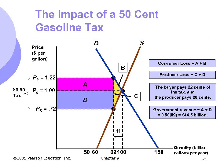
A Tax on Gasoline l We can measure the effects of a tax by looking at an example of a gasoline tax l The goal of a large gasoline tax is to: m Raise government revenue m Reduce oil consumption and reduce US dependence on oil imports l We will consider a gas tax in the market during mid-1990’s © 2005 Pearson Education, Inc. Chapter 9 53

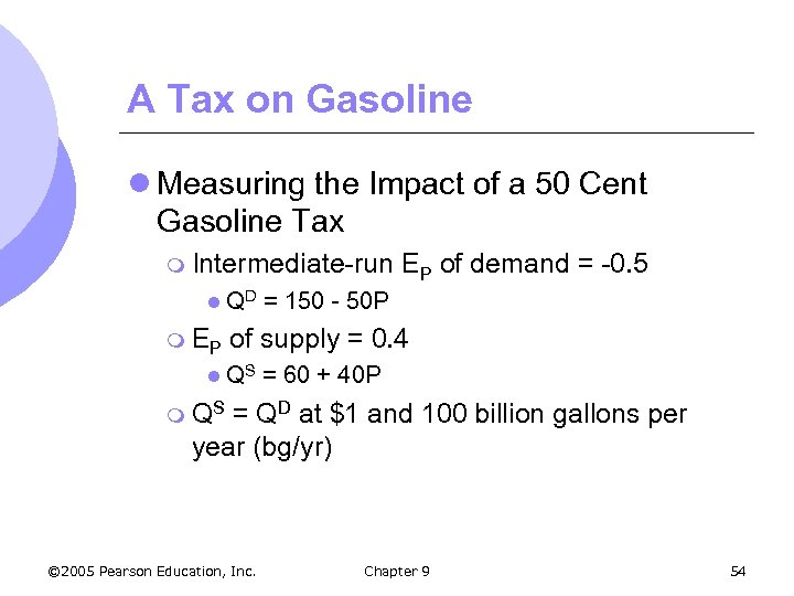A Tax on Gasoline l Measuring the Impact of a 50 Cent Gasoline Tax m Intermediate-run l QD m EP EP of demand = -0. 5 = 150 - 50 P of supply = 0. 4 l QS = 60 + 40 P m QS = QD at $1 and 100 billion gallons per year (bg/yr) © 2005 Pearson Education, Inc. Chapter 9 54

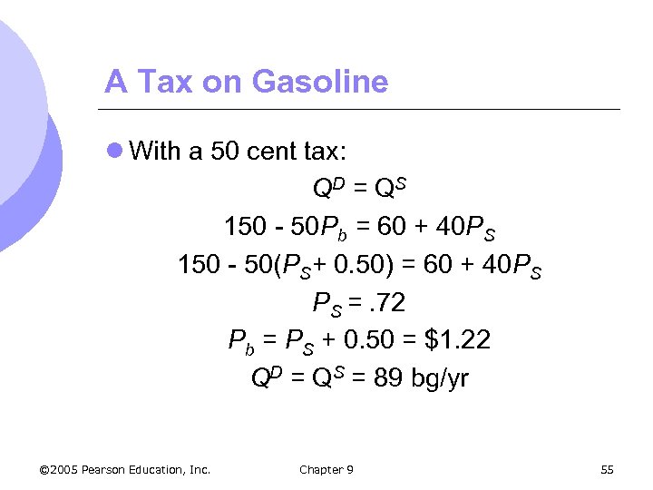A Tax on Gasoline l With a 50 cent tax: QD = QS 150 - 50 Pb = 60 + 40 PS 150 - 50(PS+ 0. 50) = 60 + 40 PS PS =. 72 Pb = PS + 0. 50 = $1. 22 QD = QS = 89 bg/yr © 2005 Pearson Education, Inc. Chapter 9 55

A Tax on Gasoline l With a 50 cent tax: m. Q falls by 11% m Price to consumers increases by 22 cents per gallon m Producers receive about 28 cents per gallon less m Both producers and consumers were opposed to the tax m Government revenue would be significant at $44. 5 billion per year © 2005 Pearson Education, Inc. Chapter 9 56

The Impact of a 50 Cent Gasoline Tax D Price ($ per gallon) S Consumer Loss = A + B B Pb = 1. 22 $0. 50 Tax P 0 = 1. 00 Producer Loss = C + D A C D PS =. 72 The buyer pays 22 cents of the tax, and the producer pays 28 cents. Government revenue = A + D = 0. 50(89) = $44. 5 billion. 11 50 60 © 2005 Pearson Education, Inc. 89 100 Chapter 9 150 Quantity (billion gallons per year) 57