ead2d9de74e104790c3c6d2d407e34d0.ppt
- Количество слайдов: 31
 Chapter 9 Properties and Applications of the Competitive Model No more good must be attempted than the public can bear. Thomas Jefferson
 Chapter 9 Outline Challenge: Licensing Taxis 9. 1 Zero Profit for Competitive Firms in the Long Run 9. 2 Producer Surplus 9. 3 Competition Maximizes Welfare 9. 4 Policies That Shift Supply Curves 9. 5 Policies That Create a Wedge Between Supply and Demand Curves 9. 6 Comparing Both Types of Policies: Trade Challenge Solution Copyright © 2014 Pearson Education, Inc. All rights reserved. 9 -2
 Challenge: Licensing Taxis • Background: • Cities around the world—including most major U. S. , Canadian, and European cities—license and limit the number of taxicabs. • Some cities regulate the number of cabs much more strictly than others. • Questions: • What effect does restrictive licensing have on taxi fares and cab company profits? • What determines the value of a license? How much profit beyond the cost of the license can the acquiring firm expect? • What are the effects of licensing on cab drivers and customers? Copyright © 2014 Pearson Education, Inc. All rights reserved. 9 -3
 9. 1 Zero Profit for Competitive Firms in the Long Run: Free Entry • With Free Entry into the Market • Along with identical costs and constant input prices, implies firms each face a horizontal LR supply curve • Firms operate at minimum LR average cost • Firms earn zero economic profit in the LR Copyright © 2014 Pearson Education, Inc. All rights reserved. 9 -4
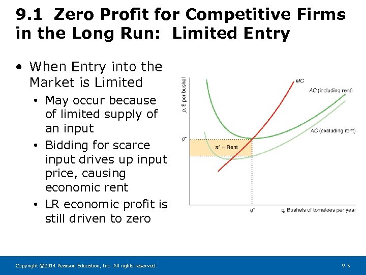 9. 1 Zero Profit for Competitive Firms in the Long Run: Limited Entry • When Entry into the Market is Limited • May occur because of limited supply of an input • Bidding for scarce input drives up input price, causing economic rent • LR economic profit is still driven to zero Copyright © 2014 Pearson Education, Inc. All rights reserved. 9 -5
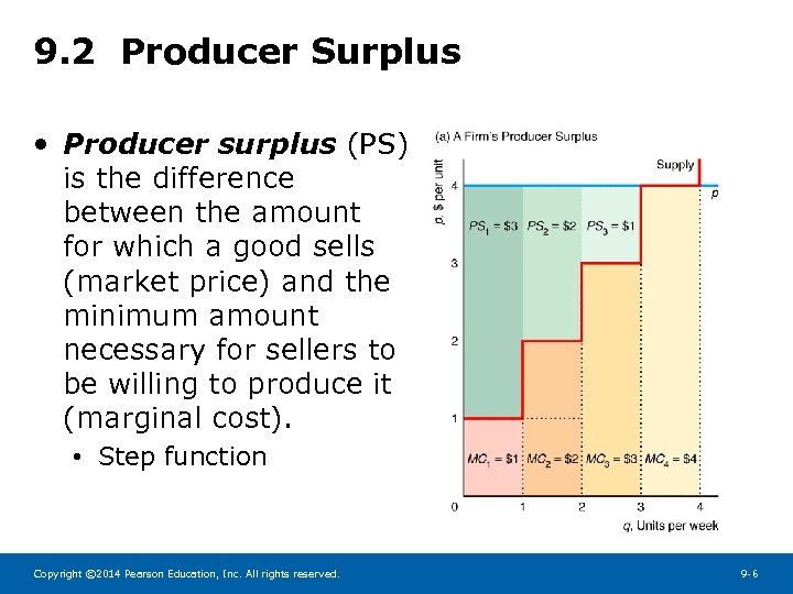 9. 2 Producer Surplus • Producer surplus (PS) is the difference between the amount for which a good sells (market price) and the minimum amount necessary for sellers to be willing to produce it (marginal cost). • Step function Copyright © 2014 Pearson Education, Inc. All rights reserved. 9 -6
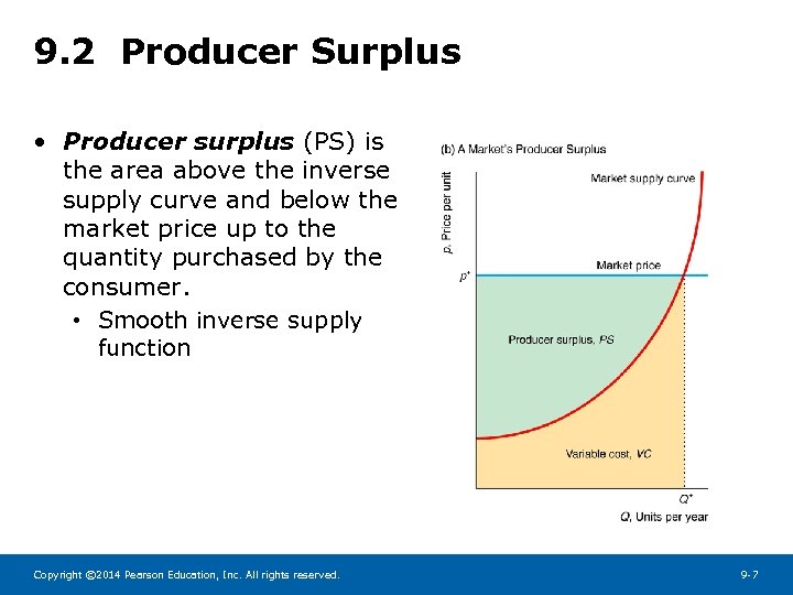 9. 2 Producer Surplus • Producer surplus (PS) is the area above the inverse supply curve and below the market price up to the quantity purchased by the consumer. • Smooth inverse supply function Copyright © 2014 Pearson Education, Inc. All rights reserved. 9 -7
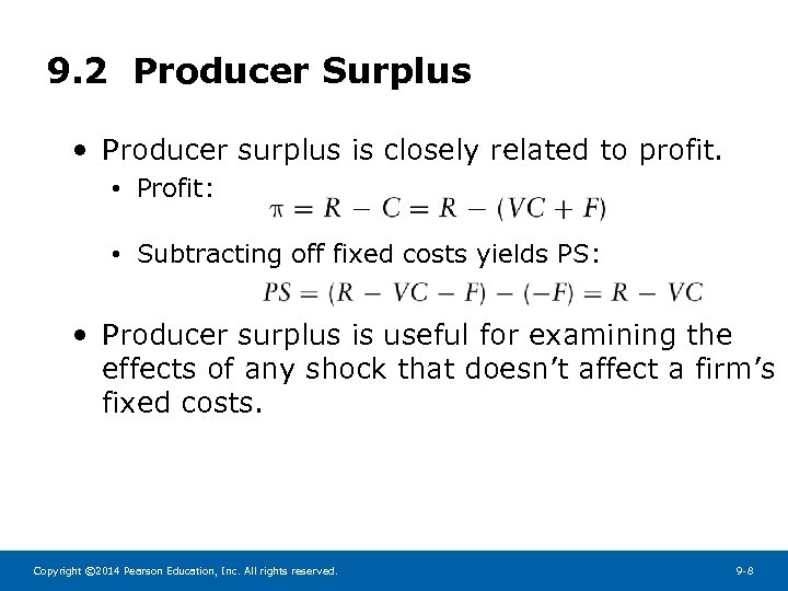 9. 2 Producer Surplus • Producer surplus is closely related to profit. • Profit: • Subtracting off fixed costs yields PS: • Producer surplus is useful for examining the effects of any shock that doesn’t affect a firm’s fixed costs. Copyright © 2014 Pearson Education, Inc. All rights reserved. 9 -8
 9. 3 Competition Maximizes Welfare • How should we measure society’s welfare? • If we are agree to weighting the well-being of consumers and producers equally, then welfare can be measured W = CS + PS • Producing the competitive quantity maximizes welfare. • Put another way, producing less than the competitive level of output lowers total welfare. • Deadweight loss (DWL) is the name for the net reduction in welfare from the loss of surplus by one group that is not offset by a gain to another group. Copyright © 2014 Pearson Education, Inc. All rights reserved. 9 -9
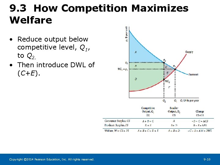 9. 3 How Competition Maximizes Welfare • Reduce output below competitive level, Q 1, to Q 2. • Then introduce DWL of (C+E). Copyright © 2014 Pearson Education, Inc. All rights reserved. 9 -10
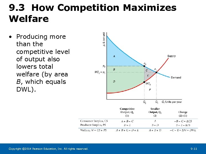 9. 3 How Competition Maximizes Welfare • Producing more than the competitive level of output also lowers total welfare (by area B, which equals DWL). Copyright © 2014 Pearson Education, Inc. All rights reserved. 9 -11
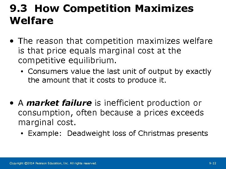 9. 3 How Competition Maximizes Welfare • The reason that competition maximizes welfare is that price equals marginal cost at the competitive equilibrium. • Consumers value the last unit of output by exactly the amount that it costs to produce it. • A market failure is inefficient production or consumption, often because a prices exceeds marginal cost. • Example: Deadweight loss of Christmas presents Copyright © 2014 Pearson Education, Inc. All rights reserved. 9 -12
 9. 4 Policies That Shift Supply Curves • Welfare is maximized at the competitive equilibrium • Government actions can move us away from that competitive equilibrium • Thus, welfare analysis can help us predict the impact of various government programs • We will examine several policies that shift supply: 1. Restricting the number of firms 2. Raising entry and exit costs Copyright © 2014 Pearson Education, Inc. All rights reserved. 9 -13
 9. 4 Policies That Shift Supply Curves • Entry Barriers: raising entry costs • A LR barrier to entry is an explicit restriction or a cost that applies only to potential new firms (e. g. large sunk costs). • Indirectly restricts the number of firms entering • Costs of entry (e. g. fixed costs of building plants, buying equipment, advertising a new product) are not barriers to entry because all firms incur them. • Exit Barriers: raising exit costs • In SR, exit barriers keep the number of firms high • In LR, exit barriers limit the number of firms entering • Example: job termination laws Copyright © 2014 Pearson Education, Inc. All rights reserved. 9 -14
 9. 5 Policies That Create a Wedge Between Supply and Demand Curves • Welfare is maximized at the competitive equilibrium • Government actions can move us away from that competitive equilibrium • Thus, welfare analysis can help us predict the impact of various government programs • We will examine several policies that create a wedge between S and D: 1. Sales tax 2. Price floor 3. Price ceiling Copyright © 2014 Pearson Education, Inc. All rights reserved. 9 -15
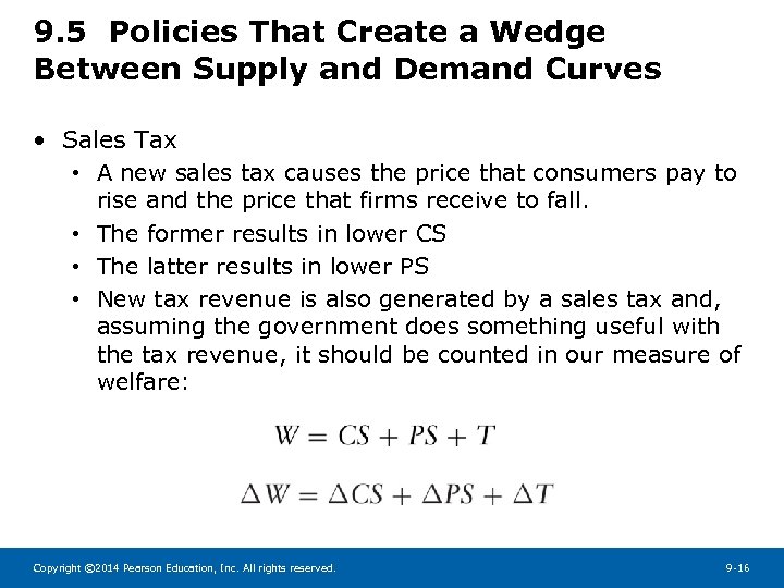 9. 5 Policies That Create a Wedge Between Supply and Demand Curves • Sales Tax • A new sales tax causes the price that consumers pay to rise and the price that firms receive to fall. • The former results in lower CS • The latter results in lower PS • New tax revenue is also generated by a sales tax and, assuming the government does something useful with the tax revenue, it should be counted in our measure of welfare: Copyright © 2014 Pearson Education, Inc. All rights reserved. 9 -16
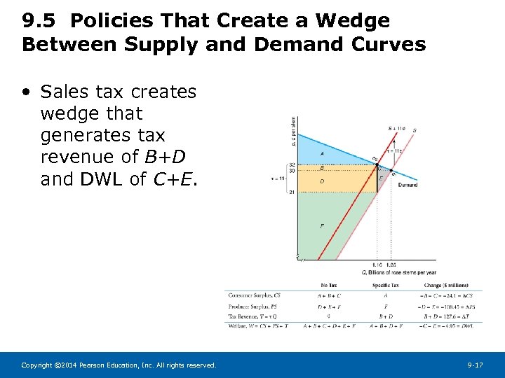 9. 5 Policies That Create a Wedge Between Supply and Demand Curves • Sales tax creates wedge that generates tax revenue of B+D and DWL of C+E. Copyright © 2014 Pearson Education, Inc. All rights reserved. 9 -17
 9. 5 Policies That Create a Wedge Between Supply and Demand Curves • Price Floor • A price floor, or minimum price, is the lowest price a consumer can legally pay for a good. • Example: agricultural products • Minimum price is guaranteed by government, but is only binding if it is above the competitive equilibrium price. • Deadweight loss generated by a price floor reflects two distortions in the market: 1. Excess production: More output is produced than consumed 2. Inefficiency in consumption: Consumers willing to pay more for last unit bought than it cost to produce Copyright © 2014 Pearson Education, Inc. All rights reserved. 9 -18
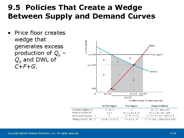 9. 5 Policies That Create a Wedge Between Supply and Demand Curves • Price floor creates wedge that generates excess production of Qs – Qd and DWL of C+F+G. Copyright © 2014 Pearson Education, Inc. All rights reserved. 9 -19
 9. 5 Policies That Create a Wedge Between Supply and Demand Curves • Price Ceiling • A price ceiling, or maximum price, is the highest price a firm can legally charge. • Example: rent controlled apartments • Maximum price is only binding if it is below the competitive equilibrium price. • Deadweight loss may underestimate true loss for two reasons: 1. Consumers spend additional time searching and this extra search is wasteful and often unsuccessful. 2. Consumers who are lucky enough to buy may not be the consumers who value it the most (allocative cost). Copyright © 2014 Pearson Education, Inc. All rights reserved. 9 -20
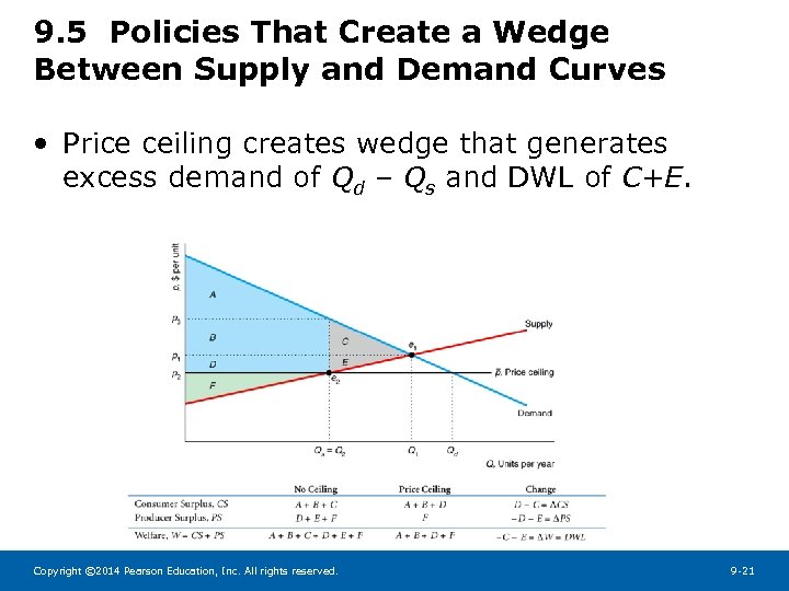 9. 5 Policies That Create a Wedge Between Supply and Demand Curves • Price ceiling creates wedge that generates excess demand of Qd – Qs and DWL of C+E. Copyright © 2014 Pearson Education, Inc. All rights reserved. 9 -21
 9. 4 Comparing Both Types of Policies: Trade • Finally, we use welfare analysis to examine government policies that are used to control international trade: 1. Free trade 2. Ban on imports (no trade) 3. Set a tariff 4. Set a quota • Welfare under free trade serves as the baseline for comparison to effects of no trade, quotas and tariffs. • Assume zero transportation costs and horizontal supply curve for the potentially imported good • Assumptions imply U. S. can import as much as it wants at p* per unit. Copyright © 2014 Pearson Education, Inc. All rights reserved. 9 -22
 9. 4 Comparing Both Types of Policies: Trading Crude Oil • Daily domestic (U. S. ) demand: • Daily domestic (U. S. ) supply: • Foreign supply curve is horizontal at the prevailing world price of $14. 70 per barrel. • Comparison of free trade and no trade (e. g. total ban on imports of crude oil) demonstrates the welfare benefit to society of free trade. Copyright © 2014 Pearson Education, Inc. All rights reserved. 9 -23
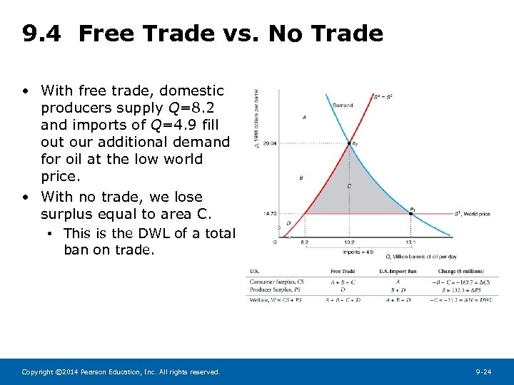 9. 4 Free Trade vs. No Trade • With free trade, domestic producers supply Q=8. 2 and imports of Q=4. 9 fill out our additional demand for oil at the low world price. • With no trade, we lose surplus equal to area C. • This is the DWL of a total ban on trade. Copyright © 2014 Pearson Education, Inc. All rights reserved. 9 -24
 9. 4 Tariffs • A tariff is essentially a tax on imports and there are two common types: • Specific tariff is a per unit tax • Ad valorem tariff is a percent of the sales price • Assuming the U. S. government institutes a tariff on foreign crude oil: 1. Tariffs protect American producers of crude oil from foreign competition. 2. Tariffs also distort American consumers’ consumption by inflating the price of crude oil. Copyright © 2014 Pearson Education, Inc. All rights reserved. 9 -25
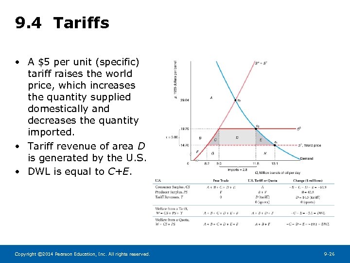 9. 4 Tariffs • A $5 per unit (specific) tariff raises the world price, which increases the quantity supplied domestically and decreases the quantity imported. • Tariff revenue of area D is generated by the U. S. • DWL is equal to C+E. Copyright © 2014 Pearson Education, Inc. All rights reserved. 9 -26
 9. 4 Quotas • A quota is a restriction on the amount of a good that can be imported. • When analyzed graphically, a quota looks very similar to a tariff. • A tariff is a restriction on price • A quota is a restriction on quantity • One can find a tariff and a quota that generate the same equilibrium • The only difference is that quotas do not generate any additional revenue for the domestic government. Copyright © 2014 Pearson Education, Inc. All rights reserved. 9 -27
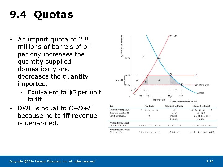 9. 4 Quotas • An import quota of 2. 8 millions of barrels of oil per day increases the quantity supplied domestically and decreases the quantity imported. • Equivalent to $5 per unit tariff • DWL is equal to C+D+E because no tariff revenue is generated. Copyright © 2014 Pearson Education, Inc. All rights reserved. 9 -28
 9. 4 Rent Seeking • Welfare analysis reveals that tariffs and quotas hurt the importing country, so why do countries continue to use these trade restrictions widely? • Domestic producers stand to make large gains from such government actions, so they organize and lobby effectively. • These efforts and expenditures to gain a rent (or profit) from government action are called rent seeking behaviors. • Although losses to all consumers are quite large, losses to any single consumer are usually small, so consumers rarely lobby against trade restrictions. Copyright © 2014 Pearson Education, Inc. All rights reserved. 9 -29
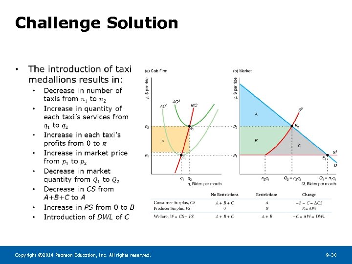 Challenge Solution • Copyright © 2014 Pearson Education, Inc. All rights reserved. 9 -30
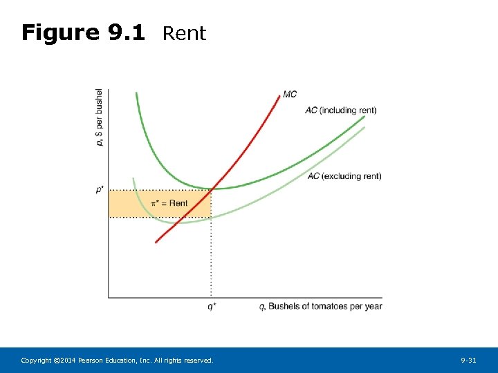 Figure 9. 1 Rent Copyright © 2014 Pearson Education, Inc. All rights reserved. 9 -31


