Chapter 9 Applying the Competitive Model 2004

Chapter 9 Applying the Competitive Model © 2004 Thomson Learning/South-Western

Consumer Surplus l l 2 Consumer surplus is the extra value individuals receive from consuming a good over what they pay for it. Alternatively, it is what people would be willing to pay for the right to consume a good at its current price.

Consumer Surplus l l l 3 In Figure 9. 1, the equilibrium price and quantity are P* and Q*. The demand curve, D, shows what people are willing to pay for the good. The total value of the good to buyers is given by the area below the demand curve from Q = 0 to Q = Q* (AEQ*0).

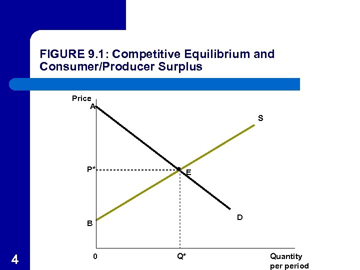FIGURE 9. 1: Competitive Equilibrium and Consumer/Producer Surplus Price A S P* E D B 4 0 Q* Quantity period

Consumer Surplus l l 5 Consumers expenditures for Q* are given by the area P*EQ*0. Consumers receive a “surplus” (total value less what they pay) equal to the area AEP*, which is shaded gray in Figure 9. 1.

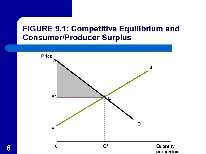FIGURE 9. 1: Competitive Equilibrium and Consumer/Producer Surplus Price A S P* E D B 6 0 Q* Quantity period

Producer Surplus l l 7 Producer surplus is the extra value producers get for a good in excess of the opportunity costs they incur for producing it. It can also be defined as what all producers would pay for the right to sell a good at its current market price.

Producer Surplus l l 8 At the equilibrium shown in Figure 9. 1, producers receive total revenue equal to the area P*EQ*0. If producers sold one unit at a time at the lowest possible price, producers would have been willing to produce Q* for the payment of BEQ*0.

Producer Surplus l 9 Thus, producer surplus the area P*EB shaded in green in Figure 9. 1.

FIGURE 9. 1: Competitive Equilibrium and Consumer/Producer Surplus Price A S P* E D B 10 0 Q* Quantity period

Short-Run Producer Surplus l l 11 The positive slope of the short-run supply curve, S, in Figure 9. 1 results from the diminishing returns to variable inputs that are encountered as output is increased. For production up to Q*, price exceeds marginal cost, so total short-run profits equal the area P*EB less fixed costs

Short-Run Producer Surplus l l l 12 Producer surplus, the area P*EB, reflects the sum of total short-run profits and short-run fixed costs. Short-run producer surplus is the part of total profits that is in excess of the profits firms would have if they chose to produce nothing at all. As such, it is similar to consumer surplus.

Long-Run Producer Surplus l l 13 Since long-run economic profits are zero and there are no fixed costs in the long-run, producer surplus is much different in the long run. The positive slope of the long-run supply curve reflects increasing input costs as output is expanded.

Long-Run Producer Surplus l l l 14 Consider the area P*EB in Figure 9. 1 as longrun producer surplus. It measures all of the increased payments relative to the situation in which the industry produces no output. The inputs would have received lower prices if this industry had not produced output.

Ricardian Rent l l 15 Ricardian rent is the long-run profits earned by owners of low-cost firms. It may be capitalized into the prices of these firms’ inputs. Assume there are many parcels of land on which tomatoes might be grown. These farms range from very fertile land (low cost) to poor, dry land (high cost).

Ricardian Rent l l l 16 At low prices, only the most fertile land is used. As output increases, higher-cost plots of land are brought into production because higher prices make this land profitable. The long-run supply curve is positively sloped because of the increasing costs associated with using less fertile land.

Ricardian Rent l l l 17 The market equilibrium price and quantity, P*, Q*, are shown in Figure 9. 2 (d). Low-cost farms, Figure 9. 2 (a) and mediumcost farms, Figure 9. 2 (b), earn long-run economic profits. Marginal farms, Figure 9. 2 (c) earn zero economic profits

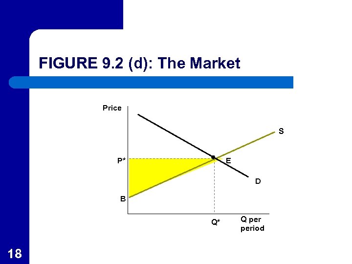FIGURE 9. 2 (d): The Market Price S P* E D B Q* 18 Q period

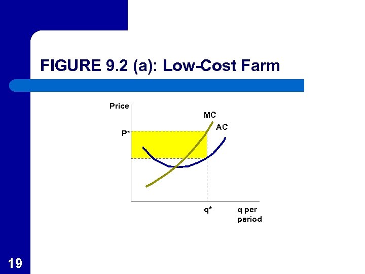FIGURE 9. 2 (a): Low-Cost Farm Price P* MC AC q* 19 q period

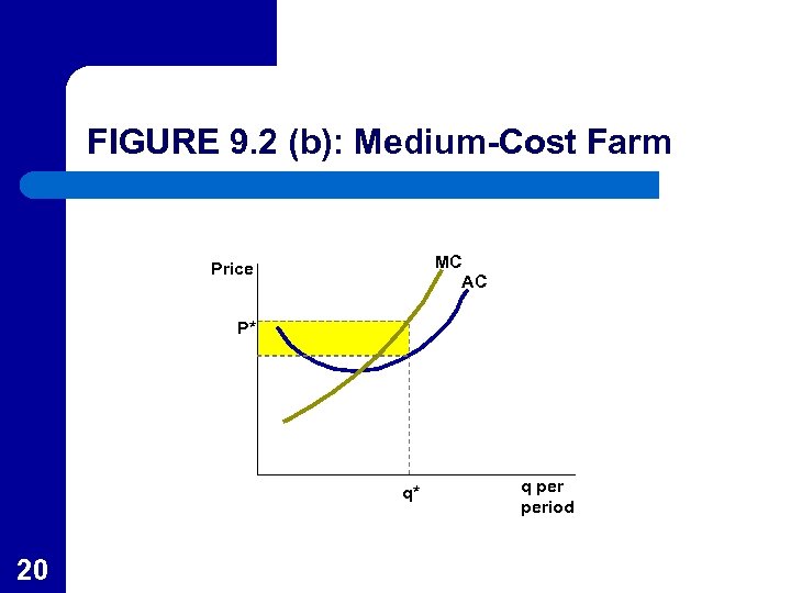FIGURE 9. 2 (b): Medium-Cost Farm MC AC Price P* q* 20 q period

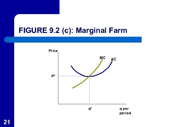FIGURE 9. 2 (c): Marginal Farm Price MC AC P* q* 21 q period

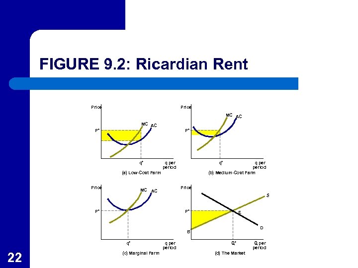FIGURE 9. 2: Ricardian Rent Price MC AC P* q* P* q period q* q period (b) Medium-Cost Farm (a) Low-Cost Farm Price MC AC S P* P* E D B q* 22 (c) Marginal Farm q period Q* (d) The Market Q period

Ricardian Rent l l l 23 Profits earned by the intramarginal farms can persist in the long run because they reflect the returns to a scarce resource, low-cost land. Entry can not erode these profits because of the scarcity of the low-cost land. The sum of these long run profits (P*EB) is the producer surplus ( Ricardian rent).

Economic Efficiency l l The competitive equilibrium is efficient in that it produces the largest surplus equal to the sum of producer and consumer surplus. In Figure 9. 1, an output level of Q 1 results in a loss of surplus equal to the area FEG. – 24 Consumers would be willing to pay P 1 for a good that producers are willing to produce for P 2, so mutually beneficial transactions exit.

FIGURE 9. 1: Competitive Equilibrium and Consumer/Producer Surplus Price A S P 1 F P* P 2 E G D B 25 0 Q 1 Q* Quantity period

APPLICATION 9. 1: Does Buying Things on the Internet Improve Welfare? l Transaction costs associated with conducting business on the internet have been reduced due to – – l 26 Technical innovations significant network externalities. Prior to this, transaction costs exceed the difference between consumers’ willingness to pay and producers costs.

APPLICATION 9. 1: Does Buying Things on the Internet Improve Welfare? l l 27 Prior to the decline in internet costs, transaction costs exceeded P 2 - P 1 in Figure 1, so no transactions occurred. Assuming transaction costs fell to zero, trading would start and a competitive equilibrium would occur at P*, Q*.

FIGURE 1: Reduced Transaction Costs Promote Internet Commerce Price P 2 S P* P 1 D 28 Q* Quantity

APPLICATION 9. 1: Does Buying Things on the Internet Improve Welfare? l Some early evidence – – – 29 Electronic retailing directly to consumers totaled about $20 billion in 2001. Business to business sales represented another $50 to $75 billion. Most sales are in travel-related goods, on-line financial services, and some narrow categories of consumer goods such as books.

APPLICATION 9. 1: Does Buying Things on the Internet Improve Welfare? l Retailers as Infomediaries – The role for retailing “middlemen” on the internet is to provide information to the consumer. l l 30 Internet automobile sellers provide comparative information about the features of cars and point to dealers with the best price. Internet airline services search for the lowest price or most convenient departure.

A Numerical Example l l l 31 The market equilibrium is P* = $6 and Q* = 4. The equilibrium is shown as point E in Figure 9. 3. At point E consumers are spending $24 ($6· 4).

A Numerical Example l l 32 At point E in Figure 9. 3, consumer surplus is $8 (= ½·$4· 4). Producers also gain a producer surplus of $8 at point E. Total consumer and producer surplus is $16. If price stays at $6 but output falls to 3, total surplus falls to $15.

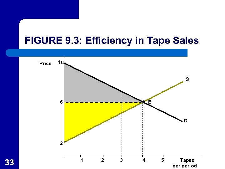FIGURE 9. 3: Efficiency in Tape Sales Price 10 S 6 E D 2 33 1 2 3 4 5 Tapes period

A Numerical Example l l 34 For any output level, total surplus is the area between the demand supply curves out to that level of output. Once output is specified, the price affects the distribution of the surplus between producers and consumers, but does not affect the total amount of the surplus.

A Numerical Example l If output > 4 tapes period with P = $6, total surplus is less than $16. – At Q = 5, consumer surplus falls to $7. 50. l l – 35 $8 for four tapes less $. 50 because the fifth tapes sells for more than people want to pay for the fifth tape. Producer surplus also equals $7. 50 reflecting the loss of $. 50 on the production of the fifth tape. Total surplus is $15 for Q = 5 tapes per week.

Price Controls and Shortages l l In Figure 9. 4 the market initially is in equilibrium at P 1, Q 1 (point E). Then demand increases from D to D’. – – 36 This would cause price to rise to P 2 encouraging entry in the short-run. Eventually entry would bring the price down to P 3 and the market would be in long-run equilibrium.

FIGURE 9. 4: Price Controls and Shortages Price SS LS P 1 E D 37 Q 1 Quantity period

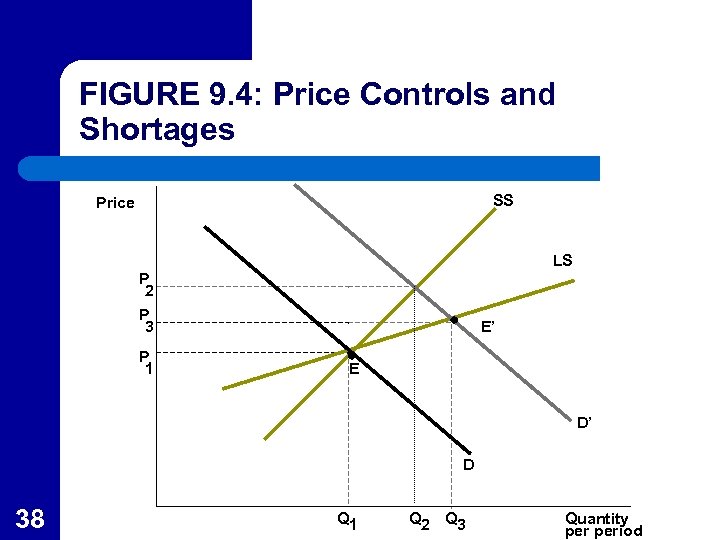FIGURE 9. 4: Price Controls and Shortages SS Price LS P 2 P 3 P 1 E’ E D’ D 38 Q 1 Q 2 Q 3 Quantity period

Price Controls and Shortages l l l 39 Suppose the government imposed a price control at the below equilibrium price of P 1 when demand increased. Firms would only supply Q 1 and no entry would take place. Since customers would demand Q 4 at this price, there would be a shortage of Q 4 - Q 1.

Price Controls and Shortages l l The welfare consequences of price control can be analyzed using consumer and producer surplus. Consumers would gain surplus of P 3 CEP 1 (colored in gray) due to the lower price. – 40 This is a direct transfer of surplus from producers to consumers with no gain in total surplus.

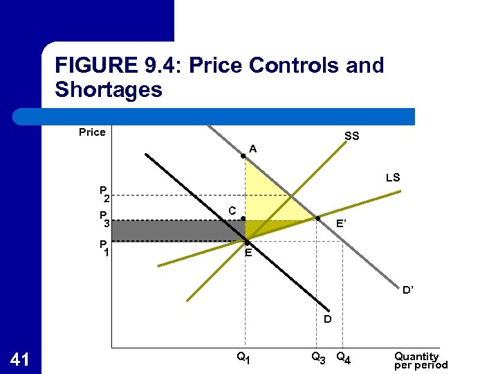FIGURE 9. 4: Price Controls and Shortages Price SS A LS P 2 P 3 P 1 C E’ E D’ D 41 Q 3 Q 4 Quantity period

Price Controls and Shortages l If output had expanded, consumers would gain the area AE’C. – l l 42 Since output is reduced by the price control, this is a loss of surplus to consumers. Similarly, producers don’t gain the area CE’E that would have resulted from increased output. The area AE’E is the total welfare loss.

Application 9. 2: Rent Control: Why This Bad Idea Never Dies l History of Rent Control – – – 43 Controls were adopted in man U. S. and European cities in response to rapidly rising rents during World War II which continued after the war in several European countries and New York City. Inflation of the 1970 s resulted in several U. S. cities introducing more “flexible” rent controls More than 10 percent of U. S. rentals are controlled.

Application 9. 2: Rent Control: Why This Bad Idea Never Dies l Rent Control and Housing Quality – – 44 Studies have confirmed the prediction that rent controls will benefit current tenants and harm landlords and new tenants. However, the most important effect is that landlords effectively reduce the supply of housing by reducing the quality of their units.

Application 9. 2: Rent Control: Why This Bad Idea Never Dies l Effects of the “New” Rent Control Laws – – – 45 By allowing landlords to pass on increases in taxes or utility costs, post World War II laws were more flexible. Many also allow rents to be increased to market levels when current tenants leave. Some economists suggest that such laws help to deal with the landlords market power, but few economists support this position.

Tax Incidence l l 46 The study of the final burden of a tax after considering all market reactions to it is tax incidence theory. The incidence of a “specific tax” of a fixed amount per unit of output that is imposed on all firms in a constant cost industry is illustrated in Figure 9. 5

FIGURE 9. 5: Effect of the Imposition of a Specific Tax on a Perfectly Competitive Constant Cost Industry Price SMC MC AC S’ S P 4 P 3 P 1 LS P 2 0 Tax q 2 q 1 (a) Typical Firm 47 Output 0 D D’ Q 3 Q 2 Q 1 Quantity per week (b) The Market

Tax Incidence l Since for any price, P, consumers pay the firm gets to keep P - t (where t is the per unit tax), the effect of the tax on firms can be shown as a decrease in demand. – l 48 The vertical distance between the demand curves is t. It creates a wedge between the consumers’ price, P, and the price firms receive.

Short-Run Tax Incidence l l 49 The short-run effect is to decrease output from Q 1 to Q 2, where firms receive P 2 and consumers pay P 3 (P 3 - P 2 = t). So long as P 2 is above minimum variable costs, the firm continues to produce and the tax incidence is shared by consumers, whose price increased to P 3, and by firm’s who now receive only P 2 rather than P 1.

Long-Run Tax Incidence l l l 50 Firms will not operate at a loss in the long run, so exit will take place shifting the short-run supply curve back to S’. In the new long-run equilibrium, output will return to Q 3 where the firm’s will receive P 1 again and consumers will pay P 4. The long-run tax incidence is all on the consumer although the firms pays the tax.

Long-Run Incidence with Increasing Costs l l 51 When the long-run supply curve has a positive slope, both consumers and firms pay a portion of the tax. The imposition of the tax shifts the long-run demand curve inward to D’ (as shown in Figure 9. 6) which causes the price to fall from P 1 to P 2 as some firms exit and input prices fall.

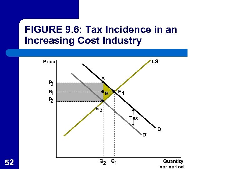FIGURE 9. 6: Tax Incidence in an Increasing Cost Industry Price P 3 P 1 P 2 LS A B E 1 E 2 Tax D D’ 52 Q 1 Quantity period

Long-Run Incidence with Increasing Costs l l l 53 Consumers pay a portion of the tax since the gross price of P 3 exceeds the pre-tax price. Total tax collection is the gray area P 3 ARE 2 P 2. The inputs to the firm pay the remainder of the tax as they are not paid based on a lower net price of P 2.

Incidence and Elasticity l The economic actor who has the most elastic curve will be able to avoid more of the tax leaving the actor with the more inelastic curve to pay most of the tax. – – 54 If demand is relatively inelastic and supply is elastic, demanders will pay most of the tax. If supply is relatively inelastic and demand is elastic, suppliers will pay most of the tax.

APPLICATION 9. 3: The Tobacco Settlement Is Just a Tax l l In November 1998 most U. S. states reached agreements with the tobacco companies that amounted to about $200 billion. The Tobacco Settlement as a Tax Increase. – – 55 This can be treated as an increase in cigarette taxes. The settlement added about $0. 30 per pack, a 15 percent increase on the initial $3. 00 price.

The Tobacco Settlement as a Tax Increase l l 56 With an elasticity of demand of -0. 35 (Table 4. 4), the quantity of cigarettes sold would be expected to fall by about 5. 25 percent (0. 35 0. 15) from 24 billion packs per year to 22. 75 billion packs. Total “tax collections” would be about $6. 8 billion per year.

The Tobacco Settlement as a Tax Increase l l l 57 If tobacco companies continue to earn about $0. 25 per pack, the 1. 25 billion reduction in sales will cost them about $300 million per year. Thus, consumers pay most of the “tax” resulting from this settlement. Since tobacco consumers tend to have relatively low incomes, the tax is regressive.

Other Effects of the Settlements l Empirical evidence suggests that young smokers may have a larger price elasticity. – – – 58 The goal of a decline in smoking by young people may be obtained. Also, studies suggest that individuals who do not smoke as teenagers are much less likely to smoke later. In addition, advertising aimed at young people was sharply restricted.

Other Effects of the Settlements l Special interest also benefited. – – – 59 Many states adopted programs to aid tobacco farmers who were affected by the decline in tobacco sales. The smallest tobacco company (Liggett) provided evidence for the states, and the higher cigarette prices will increase its profits. The lawyers who represented the states each received between $1 - $2 million per year.

Taxation and Efficiency l l 60 Taxes reduce output of the taxed commodities and a reallocation of production to other areas. Reallocation means that some mutually beneficial transactions will be foregone so economic welfare will decline.

Taxation and Efficiency l l l 61 In Figure 9. 6, the total loss of consumer surplus is the area P 3 AE 1 P 1. The area P 3 ABP 1 is transferred into tax revenue and the area AE 1 B is simply lost. The loss in producer surplus is P 1 E 1 E 2 P 2 of which P 1 BE 2 P 2 is tax revenue and BE 1 E 2 lost.

Taxation and Efficiency l l l 62 The effect of the transfer into tax revenue on welfare is ambiguous since consumers and producers may benefit from government expenditures. However, the deadweight loss is the losses of consumer and producer surplus that are not transferred to other parties. This is also called the “excess burden” of a tax.

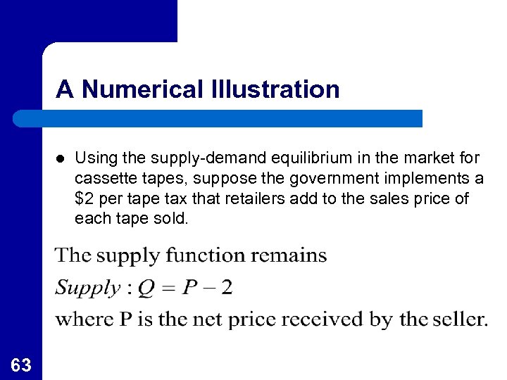A Numerical Illustration l 63 Using the supply-demand equilibrium in the market for cassette tapes, suppose the government implements a $2 per tape tax that retailers add to the sales price of each tape sold.

A Numerical Illustration l 64 Demanders, on the other hand, must pay P + t for each tape so the demand function becomes:

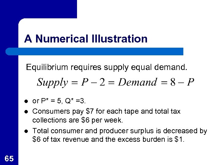A Numerical Illustration Equilibrium requires supply equal demand. l l l 65 or P* = 5, Q* =3. Consumers pay $7 for each tape and total tax collections are $6 per week. Total consumer and producer surplus is decreased by $6 of tax revenue and the excess burden is $1.

Transactions Costs l l 66 Transaction costs, such as a real estate broker fee, also cause a wedge between buyers’ and sellers’ prices. To the extent that transaction costs are on a per-unit basis, the same analysis as with a tax applies, so both parties bear some of the cost and output will be reduced.

Transactions Costs l l 67 If the wedge is a lump-sum amount per transaction, such as the cost of driving to the supermarket to buy groceries, the individual will seek to reduce the number of transactions. While prices will not change significantly, persons will hold larger inventories to reduce their transaction costs.

Gains from International Trade l l l 68 Figure 9. 7 shows the domestic demand supply curves for a particular good, say shoes. Without international trade, the equilibrium price and quantity would be PD, QD. If the world shoe price is PW, the opening of trade will cause prices to fall causing quantity to increase to Q 1.

Gains from International Trade l l The quantity supplied by domestic producers will fall to Q 2 with shoe imports of Q 1 - Q 2. Consumer surplus increases by the area P DE 0 E 1 P W. – 69 Part, PDE 0 APW, comes as a transfer from domestic producers, and the rest is an unambiguous gain in welfare (E 0 E 1 A).

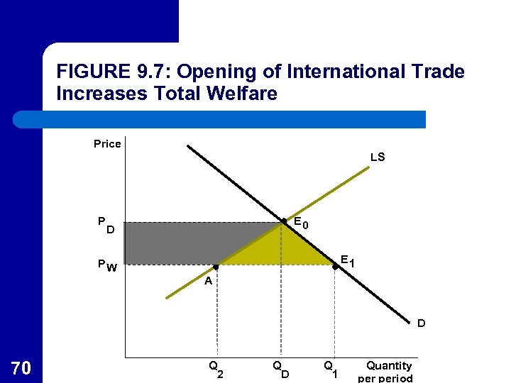FIGURE 9. 7: Opening of International Trade Increases Total Welfare Price LS P E 0 D E 1 PW A D 70 Q 2 Q D Q 1 Quantity period

Tariff Protection l l l 71 Producers will resist their losses, and since the loss is spread over fewer producers than the gain for consumers, they have a stronger incentive to organize for trade protection. A major trade protection is a tariff which is a tax on an imported good. Effects of a tariff are shown in Figure 9. 8.

FIGURE 9. 8: Effects of a Tariff Price P LS E 2 B R E 1 PW A C F D 72 Q 4 Q 3 Q 1 Quantity period

Tariff Protection l Compared to the free trade equilibrium E 1, the imposition of a per-unit tariff in the amount of t raises the effective price to PW + t = PR. – – 73 Quantity demanded falls to Q 3 while domestic production expands to Q 4. Tariff revenue is the area BE 2 FC, equal to t(Q 3 Q 4).

Tariff Protection l Total consumer surplus is reduced by the area P RE 2 E 1 P W. – – 74 Part becomes tariff revenue and part is transferred into domestic producer’s surplus (area PRBAPW). The two colored triangles BCA and E 2 E 1 F represent losses that are not transferred; these are the deadweight losses from the tariff.

Other Types of Trade Protection l l 75 Because of the General Agreement on Tariffs and Trade (GATT), there has been a decline in tariffs. However, other restrictive measures including quotas, “voluntary” export restrains, and a series of nonquantitative restrictions have been used for protectionism.

Other Types of Trade Protection l A quota that limits imports to Q 3 - Q 4 (in Figure 9. 8) would have a similar effect to a tariff. – – – 76 Market price would rise to PR. Consumer surplus would be transferred to domestic producers (area PRBAPW). A deadweight loss equal to the areas of the colored triangles would also occur.

Other Types of Trade Protection l However, with a quota, no tax revenue is generated. – l 77 The area BE 2 FC can go to foreign producers or to windfall gains to owners of import licenses. Nonquantitative restrictions such as health or other inspections also impose costs like a a tariff on imports, and can be analyzed in a similar manner using Figure 9. 8.

APPLICATION 9. 4: The Endless Saga of Steel Protectionism l l l 78 On March 6, 2002, President Bush announced that the U. S. would adopt a “temporary” tariff on steel imports. This tariff amounted to 30% on many major steel products. Other products were taxed at somewhat lower rates (8 to 15 percent).

APPLICATION 9. 4: The Endless Saga of Steel Protectionism l l It would be hard to find an industry that has had the degree of special protection from trade pressures that has characterized the U. S. steel industry. Over the past 30 years, the industry has succeeded in obtaining the following protectionist measures: – – – 79 Import quotas Minimum price agreements with exporters “Voluntary” export restraints by nations that import into the U. S.

APPLICATION 9. 4: The Endless Saga of Steel Protectionism l l l 80 Economists concluded that the costs of the 2002 tariffs to the overall economy could be quite large. Estimated tariff revenues are about $900 million annually; gains in domestic producer surplus might amount to another $700 million. Balanced against this would be estimated losses of about $2. 5 billion in consumer surplus. There might then be an annual deadweight loss of perhaps $900 million from the tariffs.