Chapter 9 AN INTRODUCTION TO ASSET PRICING MODELS

Chapter 9 AN INTRODUCTION TO ASSET PRICING MODELS

Chapter 9 Questions What are the assumptions of the capital asset pricing model? What is a risk-free asset and what are its riskreturn characteristics? What is the covariance and correlation between the risk-free asset and a risky asset or portfolio of risky assets? What is the expected return when we combine the risk-free assets and a portfolio of risky assets?

Chapter 9 Questions What is the standard deviation when we combine the risk-free asset and a portfolio of risky assets? When you combine the risk-free asset and a portfolio of risky assets on the Markowitz efficient frontier, what does the set of possible portfolios look like? Given the initial set of portfolio possibilities with a risk-free asset, what happens when you add financial leverage (that is, borrow)?

Chapter 9 Questions What is the market portfolio, what assets are included in this portfolio, and what are the relative weights for the alternative assets included? What is the capital market line (CML)? What do we mean by complete diversification? How do we measure diversification for an individual portfolio? What are systematic and unsystematic risk?

Chapter 9 Questions Given the capital market line (CML), what is the separation theorem? Given the CML, what is the relevant risk measure for an individual risky asset? What is the security market line (SML) and how does it differ from the CML? What is beta and why is it referred to as a standardized measure of systematic risk?

Chapter 9 Questions How can we use the SML to determine the expected (required) rate of return for a risky asset? Using the SML, what do we mean by an undervalued and overvalued security, and how do we determine whether an asset is undervalued or overvalued? What is an asset’s characteristic line and how do we compute the characteristic line for an asset?

Chapter 9 Questions What is the impact on the characteristic line when we compute it using different return intervals (such as weekly versus monthly) and when we employ different proxies (that is, benchmarks) for the market portfolio (for example, the S&P 500 versus a global stock index)?

Chapter 9 Questions What is the arbitrage pricing theory (APT) and how does it differ from the capital asset pricing model (CAPM) in terms of assumptions? How does the APT differ from the CAPM in terms of risk measure?

Capital Market Theory: An Overview Capital market theory extends portfolio theory and seeks to develops a model for pricing all risky assets based on their relevant risks Asset Pricing Models l l Capital asset pricing model (CAPM) allows for the calculation of the required rate of return for any risky asset based on the security’s beta Arbitrage Pricing Theory (APT) is a multi-factor model for determining the required rate of return

Assumptions of Capital Market Theory All investors are Markowitz efficient investors who invest on the efficient frontier. Investors can borrow or lend any amount of money at the risk-free rate of return (RFR). Investors have homogeneous expectations; that is, they estimate identical probability distributions for future rates of return. All investors have the same one-period time horizon such as one-month, six months, or one year.

Assumptions of Capital Market Theory All investments are infinitely divisible, which means that it is possible to buy or sell fractional shares of any asset or portfolio. There are no taxes or transaction costs involved in buying or selling assets. There is no inflation or any change in interest rates, or inflation is fully anticipated. Capital markets are in equilibrium.

Making Assumptions Some of these assumptions are clearly unrealistic Relaxing many of these assumptions would have only minor influence on the model and would not change its main implications or conclusions. The primary way to judge a theory is on how well it explains and helps predict behavior, not on its assumptions.

Capital Market Theory and a Risk-Free Asset Perhaps surprisingly, there are rather large implications for capital market theory when a risk-free asset exists. What is a risk-free asset? l l l An asset with zero variance Provides the risk-free rate of return (RFR) It will be an “intercept” value on a portfolio graph between expected return and standard deviation. Since it has zero variance, it will also have zero correlation with all other risky assets

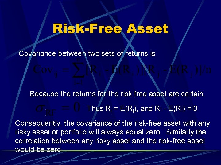Risk-Free Asset Covariance between two sets of returns is Because the returns for the risk free asset are certain, Thus Ri = E(Ri), and Ri - E(Ri) = 0 Consequently, the covariance of the risk-free asset with any risky asset or portfolio will always equal zero. Similarly the correlation between any risky asset and the risk-free asset would be zero.

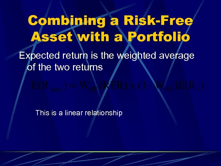Combining a Risk-Free Asset with a Portfolio Expected return is the weighted average of the two returns This is a linear relationship

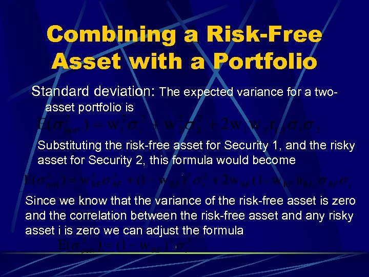Combining a Risk-Free Asset with a Portfolio Standard deviation: The expected variance for a twoasset portfolio is Substituting the risk-free asset for Security 1, and the risky asset for Security 2, this formula would become Since we know that the variance of the risk-free asset is zero and the correlation between the risk-free asset and any risky asset i is zero we can adjust the formula

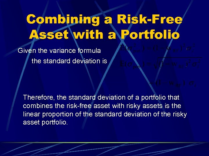Combining a Risk-Free Asset with a Portfolio Given the variance formula the standard deviation is Therefore, the standard deviation of a portfolio that combines the risk-free asset with risky assets is the linear proportion of the standard deviation of the risky asset portfolio.

Combining a Risk-Free Asset with a Portfolio Since both the expected return and the standard deviation of return for such a portfolio are linear combinations, a graph of possible portfolio returns and risks looks like a straight line between the two assets.

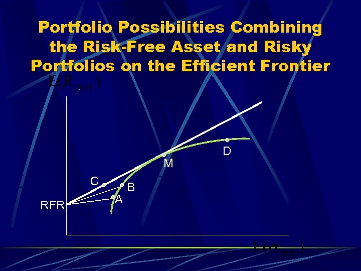Portfolio Possibilities Combining the Risk-Free Asset and Risky Portfolios on the Efficient Frontier M C RFR A B D

Risk-Return Possibilities with Leverage To attain a higher expected return than is available at point M (in exchange for accepting higher risk) Either invest along the efficient frontier beyond point M, such as point D Or, add leverage to the portfolio by borrowing money at the risk-free rate and investing in the risky portfolio at point M

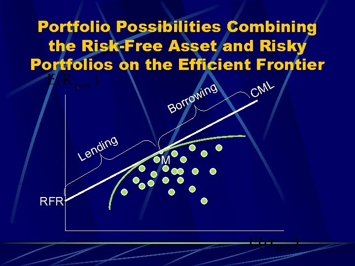Portfolio Possibilities Combining the Risk-Free Asset and Risky Portfolios on the Efficient Frontier orr B ing nd Le RFR M o ing w ML C

The Market Portfolio M lies at the point of tangency, so it has the highest portfolio possibility line This line of tangency is called the Capital Market Line (CML) Everybody will want to invest in Portfolio M and borrow or lend to be somewhere on the CML (the CML is a new efficient frontier) l Therefore this portfolio must include all risky assets (or else some assets would have no demand)

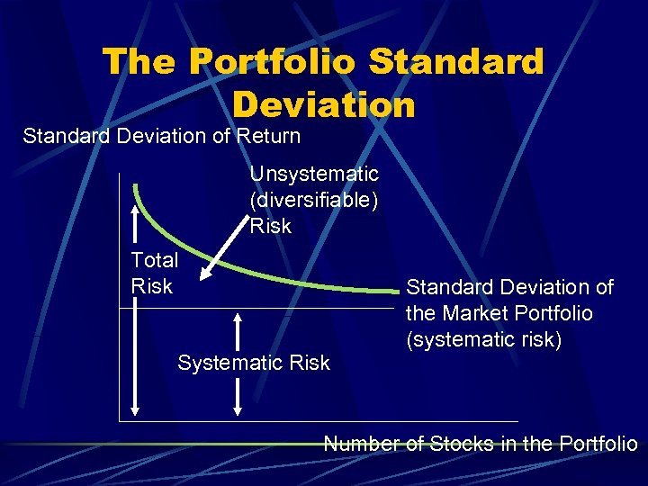
The Market Portfolio Because the market is in equilibrium, all assets are included in this portfolio in proportion to their market value Because it contains all risky assets, it is a completely diversified portfolio, which means that all the unique risk of individual assets (unsystematic risk) is diversified away

Systematic Risk Only systematic risk remains in the market portfolio Systematic risk is the variability in all risky assets caused by macroeconomic variables Systematic risk can be measured by the standard deviation of returns of the market portfolio and can change over time

Factors Affecting Systematic Risk Systematic risk factors are those macroeconomic variables that affect the valuation of all risky assets Variability in growth of the money supply l Interest rate volatility l Variability in aggregate industrial production l

How to Measure Diversification All portfolios on the CML are perfectly positively correlated with each other and with the completely diversified market Portfolio M A completely diversified portfolio would have a correlation with the market portfolio of +1. 00

Diversifying Away Unsystematic Risk The purpose of diversification is to reduce the standard deviation of the total portfolio As you add securities, you expect the average covariance for the portfolio to decline, but not to disappear since correlations are not perfectly negative. About how many securities must you add to obtain a completely diversified portfolio? l l About 90% of the benefit after 12 -18 stocks Maximum benefit needs between 30 and 40

The Portfolio Standard Deviation of Return Unsystematic (diversifiable) Risk Total Risk Systematic Risk Standard Deviation of the Market Portfolio (systematic risk) Number of Stocks in the Portfolio

The CML and the Separation Theorem The CML leads all investors to invest in the M portfolio (The Investment Decision) Individual investors should differ in position on the CML depending on risk preferences (which leads to the Financing Decision) l l Risk averse investors will lend part of the portfolio at the risk-free rate and invest the remainder in the market portfolio (points left of M) Aggressive investors would borrow funds at the RFR and invest everything in the market portfolio (points to the right of M)

A Risk Measure for the CML If… the relevant risk in a portfolio is the average covariance with all other assets in the portfolio, and … the only relevant portfolio is the market portfolio (M), then it follows that … the covariance with the market portfolio is the relevant (systematic) risk of an asset.

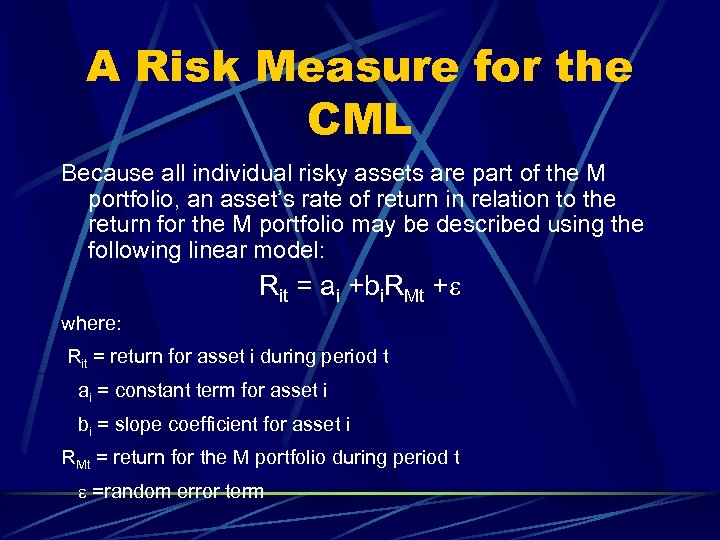A Risk Measure for the CML Because all individual risky assets are part of the M portfolio, an asset’s rate of return in relation to the return for the M portfolio may be described using the following linear model: Rit = ai +bi. RMt +e where: Rit = return for asset i during period t ai = constant term for asset i bi = slope coefficient for asset i RMt = return for the M portfolio during period t e =random error term

The Capital Asset Pricing Model The existence of a risk-free asset resulted in deriving a capital market line (CML) that became the relevant frontier An asset’s covariance with the market portfolio is the relevant risk measure This can be used to determine an appropriate required rate of return on a risky asset - the capital asset pricing model (CAPM)

The Capital Asset Pricing Model CAPM indicates what should be the expected or required rates of return on risky assets This helps to value an asset by providing an appropriate discount rate to use in dividend valuation models You can compare an expected rate of return to the required rate of return implied by CAPM - over/ under valued?

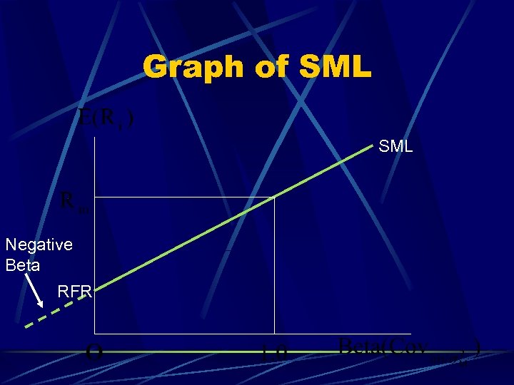
The Security Market Line (SML) The relevant risk measure for an individual risky asset is its covariance with the market portfolio (Covi, m) This is shown as the risk measure The return for the market portfolio should be consistent with its own risk, which is the covariance of the market with itself - or its variance

The Security Market Line (SML) We then define as beta

Graph of SML Negative Beta RFR

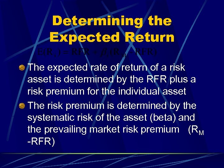Determining the Expected Return The expected rate of return of a risk asset is determined by the RFR plus a risk premium for the individual asset The risk premium is determined by the systematic risk of the asset (beta) and the prevailing market risk premium (RM -RFR)

Determining the Expected Return In equilibrium, all assets and all portfolios of assets should plot on the SML l l l The SML gives the market “going rate of return” or what you should earn as a return for a security Any security with an expected return that plots above the SML is underpriced Any security with an expected return that plots below the SML is overpriced

Identifying Undervalued and Overvalued Assets Compare the required rate of return to the expected rate of return for a specific risky asset using the SML over a specific investment horizon to determine if it is an appropriate investment Independent estimates of expected return for the securities provide price and dividend outlooks

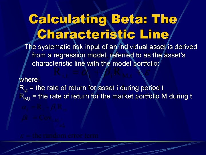Calculating Beta: The Characteristic Line The systematic risk input of an individual asset is derived from a regression model, referred to as the asset’s characteristic line with the model portfolio: where: Ri, t = the rate of return for asset i during period t RM, t = the rate of return for the market portfolio M during t

Issues in Beta Estimation The Impact of the Time Interval l Number of observations and time interval used in regression vary l l l Value Line Investment Services (VL) uses weekly rates of return over five years Merrill Lynch, Pierce, Fenner & Smith (ML) uses monthly return over five years There is no “correct” interval for analysis Weak relationship between VL & ML betas due to difference in intervals used Interval effect impacts smaller firms more

Issues in Beta Estimation The Effect of the Market Proxy l l A measure of the market portfolio is needed S&P 500 Composite Index is most often used l l l Includes a large proportion of the total market value of U. S. stocks Value weighted series Weaknesses of Using S&P 500 as the Market Proxy l l Includes only U. S. stocks The theoretical market portfolio should include all types of assets from all around the world

Arbitrage Pricing Theory (APT) CAPM is criticized because of the difficulties in selecting a proxy for the market portfolio as a benchmark An alternative pricing theory with fewer assumptions was developed: l Arbitrage Pricing Theory

Assumptions of Arbitrage Pricing Theory Capital markets are perfectly competitive Investors always prefer more wealth to less wealth with certainty The stochastic process generating asset returns can be presented as a k-factor model

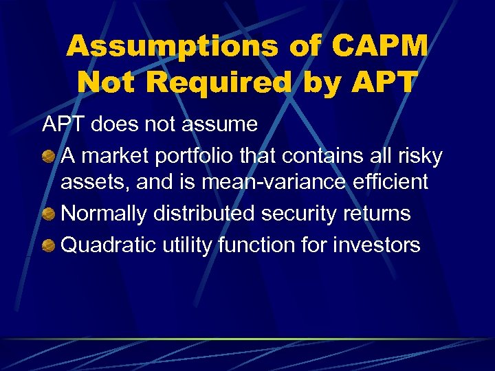Assumptions of CAPM Not Required by APT does not assume A market portfolio that contains all risky assets, and is mean-variance efficient Normally distributed security returns Quadratic utility function for investors

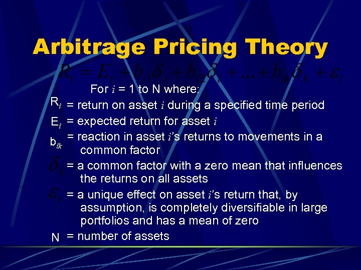Arbitrage Pricing Theory Ri Ei bik N For i = 1 to N where: = return on asset i during a specified time period = expected return for asset i = reaction in asset i’s returns to movements in a common factor = a common factor with a zero mean that influences the returns on all assets = a unique effect on asset i’s return that, by assumption, is completely diversifiable in large portfolios and has a mean of zero = number of assets

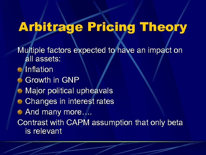Arbitrage Pricing Theory Multiple factors expected to have an impact on all assets: Inflation Growth in GNP Major political upheavals Changes in interest rates And many more…. Contrast with CAPM assumption that only beta is relevant

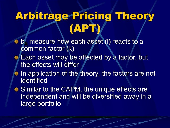Arbitrage Pricing Theory (APT) bik measure how each asset (i) reacts to a common factor (k) Each asset may be affected by a factor, but the effects will differ In application of theory, the factors are not identified Similar to the CAPM, the unique effects are independent and will be diversified away in a large portfolio

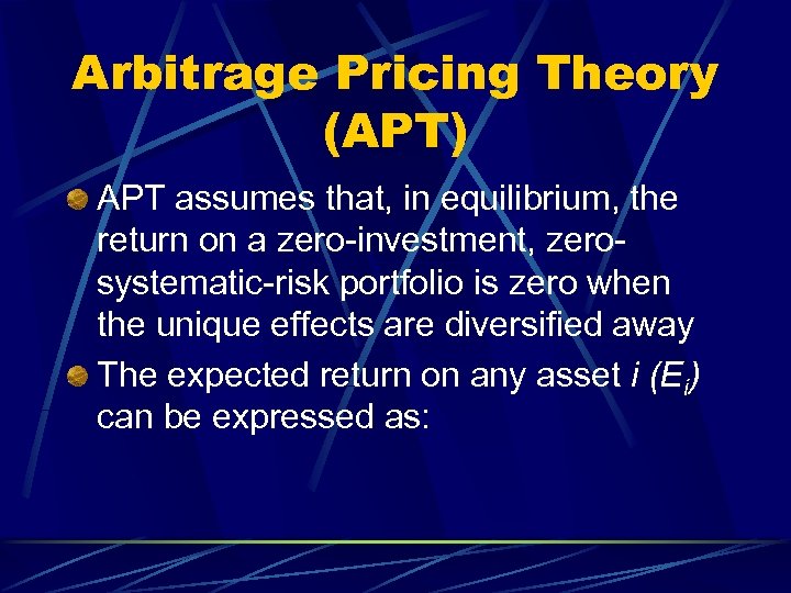Arbitrage Pricing Theory (APT) APT assumes that, in equilibrium, the return on a zero-investment, zerosystematic-risk portfolio is zero when the unique effects are diversified away The expected return on any asset i (Ei) can be expressed as:

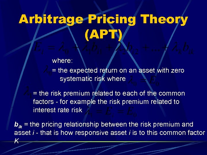Arbitrage Pricing Theory (APT) where: = the expected return on an asset with zero systematic risk where = the risk premium related to each of the common factors - for example the risk premium related to interest rate risk bik = the pricing relationship between the risk premium and asset i - that is how responsive asset i is to this common factor K

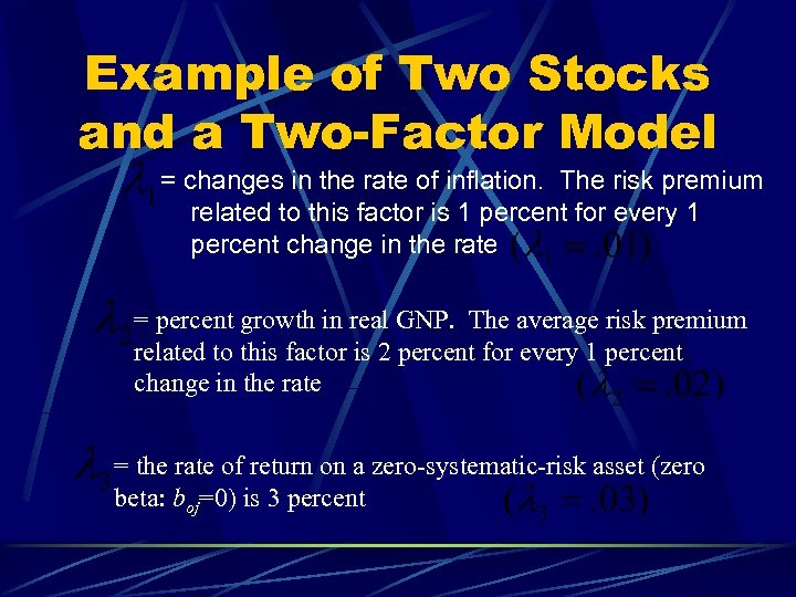Example of Two Stocks and a Two-Factor Model = changes in the rate of inflation. The risk premium related to this factor is 1 percent for every 1 percent change in the rate = percent growth in real GNP. The average risk premium related to this factor is 2 percent for every 1 percent change in the rate = the rate of return on a zero-systematic-risk asset (zero beta: boj=0) is 3 percent

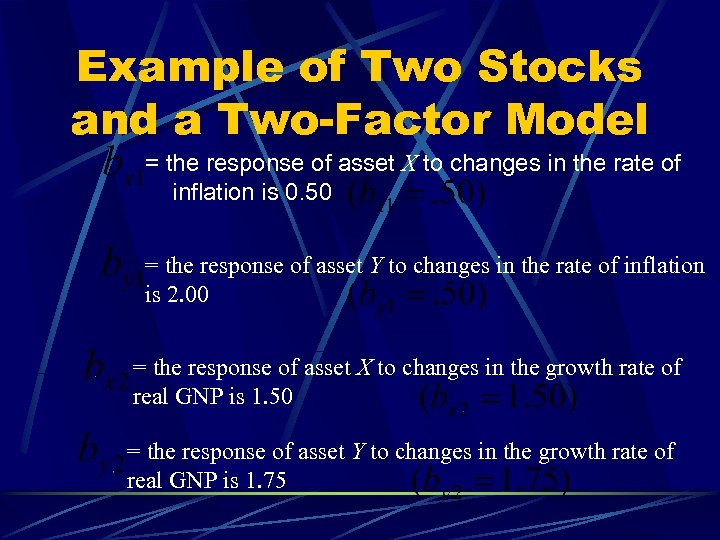Example of Two Stocks and a Two-Factor Model = the response of asset X to changes in the rate of inflation is 0. 50 = the response of asset Y to changes in the rate of inflation is 2. 00 = the response of asset X to changes in the growth rate of real GNP is 1. 50 = the response of asset Y to changes in the growth rate of real GNP is 1. 75

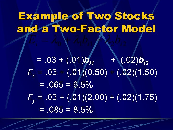Example of Two Stocks and a Two-Factor Model =. 03 + (. 01)bi 1 + (. 02)bi 2 Ex =. 03 + (. 01)(0. 50) + (. 02)(1. 50) =. 065 = 6. 5% Ey =. 03 + (. 01)(2. 00) + (. 02)(1. 75) =. 085 = 8. 5%

Empirical Tests of the APT Studies by Roll and Ross and by Chen support APT by explaining different rates of return with some better results than CAPM Reinganum’s study indicated that the APT does not explain small-firm results Dhrymes and Shanken question the usefulness of APT because it was not possible to identify the factors and therefore may not be testable