Chapter 8 Geocomputation Part A Cellular Automata CA

Chapter 8 Geocomputation Part A: Cellular Automata (CA) & Agent-based modelling (ABM) www. spatialanalysisonline. com

Geocomputation “the art and science of solving complex spatial problems with computers” www. geocomputation. org Key new areas of geocomputation: Presentation 8 A: Geosimulation (CA and ABM) Presentation 8 B: Artificial Neural Networks (ANNs); & Evolutionary computing (EC) 3 rd edition www. spatialanalysisonline. com 2

Geocomputation Many other, well-established areas: Automated zoning/re-districting (e. g. AZP) ¡ Cluster hunting (e. g. GAM/K) ¡ Interactive data mining tools (e. g. brushing and linking, cross-tabbed attribute mapping) ¡ Visualisation tools (e. g. 3 D and 4 D visualisation, immersive systems… some also very new!) ¡ Advanced raster processing (e. g. ACS/distance transforms, visibility analysis, image processing etc. ) ¡ Heuristic and metaheuristic spatial optimisation, …. and more! ¡ 3 rd edition www. spatialanalysisonline. com 3

Geocomputation: Geosimulation For the purposes of this discussion: Geosimulation includes ¡ Cellular automata (CA) ¡ Agent-based modelling (ABM) Geosimulation is particularly concerned with ¡ Researching processes ¡ Identifying and understanding emergent behaviours and outcomes ¡ Spatio-temporal modelling 3 rd edition www. spatialanalysisonline. com 4

Geocomputation: ANNs In the next presentation on geocomputation: ANNs discussed include ¡ Multi-level perceptrons (MLPs) ¡ Radial basis function neural networks (RBFNNs) ¡ Self organising feature maps (SOFMs) ANNs are particularly concerned with ¡ Function approximation and interpolation ¡ Image analysis and classification ¡ Spatial interaction modelling 3 rd edition www. spatialanalysisonline. com 5

Geocomputation: Evolutionary computing In the next presentation on geocomputation: EC elements discussed include ¡ Genetic algorithms (GAs) ¡ Genetic programming (GP) EC is particularly concerned with ¡ Complex problem solving using GAs ¡ Model design using GP methods 3 rd edition www. spatialanalysisonline. com 6

Cellular automata (CA) CA are computer based simulations that use a static cell framework or lattice as the environment (model of space) l Each cells has a well-defined state at every specific discrete point in time l Cell states may change over time according to state transition rules l Transition rules that are applied to cells depend upon their neighbourhoods (i. e. the states of adjacent cells typically) l 3 rd edition www. spatialanalysisonline. com 7

Cellular automata ¡ State variables l l ¡ Spatial framework l l ¡ l Typically Moore (8 -way) or von Neumann (4 -way) Typically lag=1 but lag=2. . and alternatives are possible Transition rules l l 3 rd edition typically a regular lattice, but could be irregular boundary issues and edge wrapping options Neighbourhood structure l ¡ typically binary (e. g. alive/dead), but can be more complex may have fixed (captured) states Typically deterministic but may be more complex Time treated as discrete steps and all operations are synchronous (parallel not sequential changes) www. spatialanalysisonline. com 8

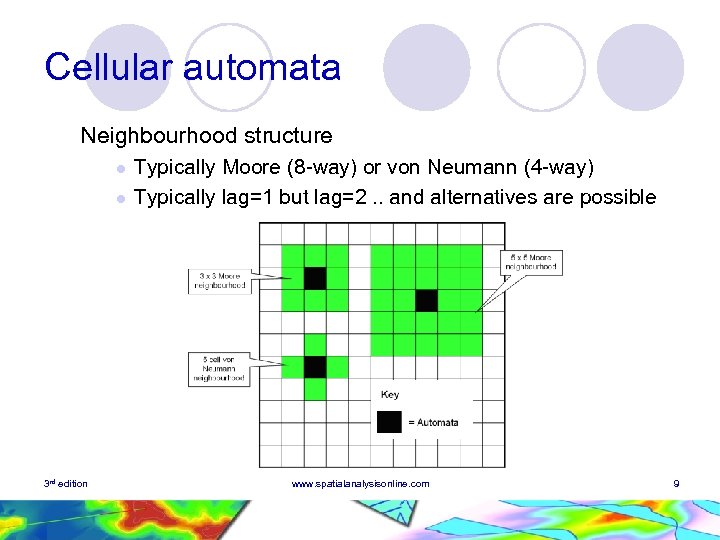Cellular automata Neighbourhood structure l l 3 rd edition Typically Moore (8 -way) or von Neumann (4 -way) Typically lag=1 but lag=2. . and alternatives are possible www. spatialanalysisonline. com 9

Cellular automata Example 1 – Game of life ¡ ¡ State variables: cells contain a 1 or a 0 (alive or dead) Spatial framework: operates over a rectangular lattice (with square cells) Neighbourhood structure: 4 adjacent (rook’s move) cells State transition rules: time tn tn+1 1. 2. 3. 3 rd edition Survival: if state=1 and in neighbourhood 2 or 3 cells have state=1 then state 1 else state 0 Reproduction: if state=0 but state=3 or 4 in neighbouring cells then state 1 Death (loneliness or overcrowding): if state=1 but state<>2 or 3 in neighbourhood then state 0 www. spatialanalysisonline. com 10

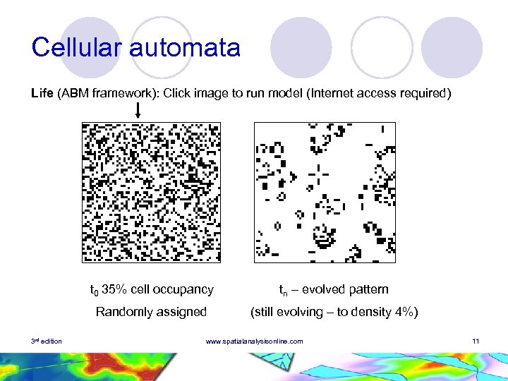Cellular automata Life (ABM framework): Click image to run model (Internet access required) t 0 35% cell occupancy Randomly assigned 3 rd edition tn – evolved pattern (still evolving – to density 4%) www. spatialanalysisonline. com 11

Cellular automata Example 2 – Heatbugs ¡ State variables: l l l ¡ State transition rules: time tn tn+1 1. 2. 3. 4. 3 rd edition Cells may be occupied by bugs or not Cells have an ambient temperature value 0 Bugs have an ideal heat (min and max rates settable) – i. e. a state of ‘happiness’ Bugs can move, but only to an adjacent cell that does not have a bug on it Bugs move if they are ‘unhappy’ – too hot or too cold (if they can move to a better adjacent cell) Bugs emit heat (min and max rates settable) Heat diffuses slowly through the grid and some is lost to ‘evaporation’ www. spatialanalysisonline. com 12

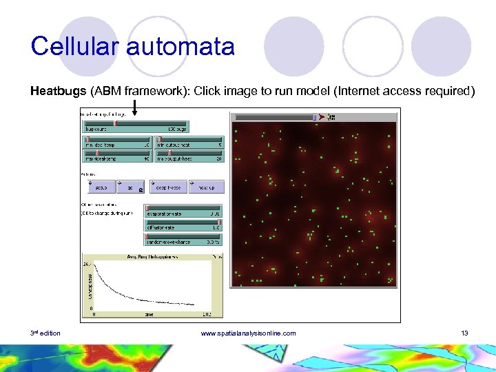Cellular automata Heatbugs (ABM framework): Click image to run model (Internet access required) 3 rd edition www. spatialanalysisonline. com 13

Cellular automata l Example geospatial modelling applications: ¡ ¡ ¡ l Bushfires Deforestation Earthquakes Rainforest dynamics Urban systems But. . ¡ ¡ 3 rd edition Not very flexible Difficult to adequately model mobile entities (e. g. pedestrians, vehicles)… interest in ABM www. spatialanalysisonline. com 14

Agent-based modelling l l Dynamic systems of multiple interacting agents Agents are complex ‘individuals’ with various primary characteristics, e. g. ¡ Autonomy, Mobility, Reactive or pro-active behaviour, Vision, Communications capabilities, Learning capabilities Operate within a model or simulation environment l Time treated synchronously or asynchronously l CA can be modelling using ABM, but reverse may be difficult l Bottom-up rather than top-down modelling l 3 rd edition www. spatialanalysisonline. com 15

Agent-based modelling l Sample applications: ¡ Archaeological reconstruction ¡ Biological models of infectious diseases ¡ Modelling economic processes ¡ Modelling political processes ¡ Traffic simulations ¡ Analysis of social networks ¡ Pedestrian modelling (crowds behaviour, evacuation modelling etc. ) … 3 rd edition www. spatialanalysisonline. com 16

Agent-based modelling l Example 1: Schelling segregation model Actually a CA model implemented here in an ABM framework. Agents represent people; agent interactions model a social process ¡ ¡ Spatial framework: Cell based State variables: grey – cell unoccupied; red – occupied by red group; black – occupied by black group Neighbourhood structure (Moore) State transition rules: l l 3 rd edition If proportion of neighbours of the same colour x% then stay where you are, else If proportion of neighbours of the same colour

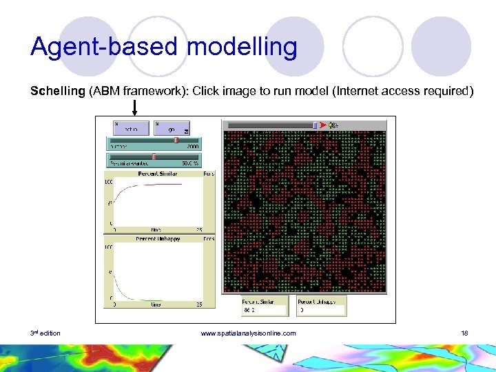Agent-based modelling Schelling (ABM framework): Click image to run model (Internet access required) 3 rd edition www. spatialanalysisonline. com 18

Agent-based modelling l Example 2: Pedestrian movement ¡ Realistic spatial framework ¡ Multiple passengers arriving and departing ¡ Multiple targets – ticket machines, ticket booths, subway platforms, mainline platforms, shop, exits … ¡ Free movement with obstacle avoidance 3 rd edition www. spatialanalysisonline. com 19

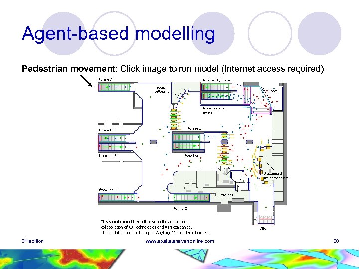Agent-based modelling Pedestrian movement: Click image to run model (Internet access required) 3 rd edition www. spatialanalysisonline. com 20

Agent-based modelling l Advantages of ABM ¡ Captures emergent phenomena l l ¡ Provides a natural environment for study l ¡ Spatial framework can be complex and realistic Flexible l 3 rd edition Interactions can be complicated, non-linear, discontinuous or discrete Populations can be heterogeneous, have differential learning patterns, different levels of rationality etc Can handle multiple scales, distance-related components, directional components, agent complexity etc www. spatialanalysisonline. com 21

Agent-based modelling l Disadvantages of/issues for ABM ¡ ¡ ¡ ¡ 3 rd edition What is the real ‘purpose’ of model? What is the appropriate scale for research? How are the results to be interpreted? How robust is the model? Can the model be replicated? Can the results be validated? Are behaviours/patterns observed likely to occur in the real world? How much is the outcome dependent on the model implementation (design, toolset, parameters etc. )? www. spatialanalysisonline. com 22

Agent-based modelling l Choosing a simulation/modelling system ¡ Ease of development ¡ Size of user community ¡ Availability of support ¡ Availability of demonstration/template models ¡ Availability of ‘how-to’ materials and documentation ¡ Licensing policy (open source, shareware/freeware, proprietary) 3 rd edition www. spatialanalysisonline. com 23

Agent-based modelling l Choosing a simulation/modelling system ¡ Key features Number of agents that can be modelled l Degree of agent-agent interaction supported l Model environments (and scale) supported (network, raster, vector) l Multi-level support (agent hierarchies) l Spatial relationships support l Event scheduling/sequencing facilities l 3 rd edition www. spatialanalysisonline. com 24

Agent-based modelling l Major simulation/modelling systems ¡ open source: SWARM, MASON, Repast ¡ shareware/freeware: Star. Logo, Net. Logo, OBEUS) ¡ proprietary systems: Agent. Sheets, Any. Logic 3 rd edition www. spatialanalysisonline. com 25