Chapter 8 EXPECTED UTILITY AND RISK AVERSION MICROECONOMIC

Chapter 8 EXPECTED UTILITY AND RISK AVERSION MICROECONOMIC THEORY BASIC PRINCIPLES AND EXTENSIONS EIGHTH EDITION WALTER NICHOLSON Copyright © 2002 by South-Western, a division of Thomson Learning. All rights reserved.

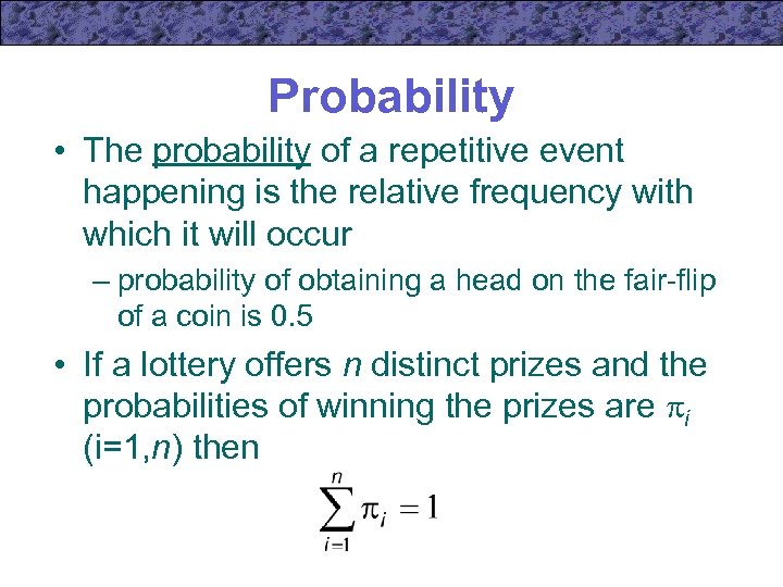Probability • The probability of a repetitive event happening is the relative frequency with which it will occur – probability of obtaining a head on the fair-flip of a coin is 0. 5 • If a lottery offers n distinct prizes and the probabilities of winning the prizes are i (i=1, n) then

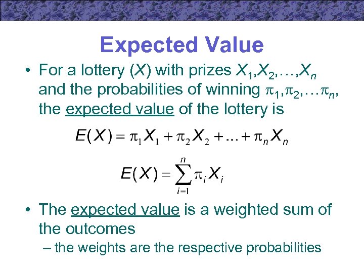Expected Value • For a lottery (X) with prizes X 1, X 2, …, Xn and the probabilities of winning 1, 2, … n, the expected value of the lottery is • The expected value is a weighted sum of the outcomes – the weights are the respective probabilities

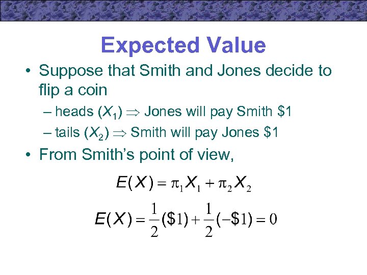Expected Value • Suppose that Smith and Jones decide to flip a coin – heads (X 1) Jones will pay Smith $1 – tails (X 2) Smith will pay Jones $1 • From Smith’s point of view,

Expected Value • Games which have an expected value of zero (or cost their expected values) are called actuarially fair games – a common observation is that people often refuse to participate in actuarially fair games

Fair Games • People are generally unwilling to play fair games • There may be a few exceptions – when very small amounts of money are at stake – when there is utility derived from the actual play of the game • we will assume that this is not the case

St. Petersburg Paradox • A coin is flipped until a head appears • If a head appears on the nth flip, the player is paid $2 n X 1 = $2, X 2 = $4, X 3 = $8, …, Xn = $2 n • The probability of getting a head on the ith trial is (½)i 1=½, 2= ¼, …, n=(½)n

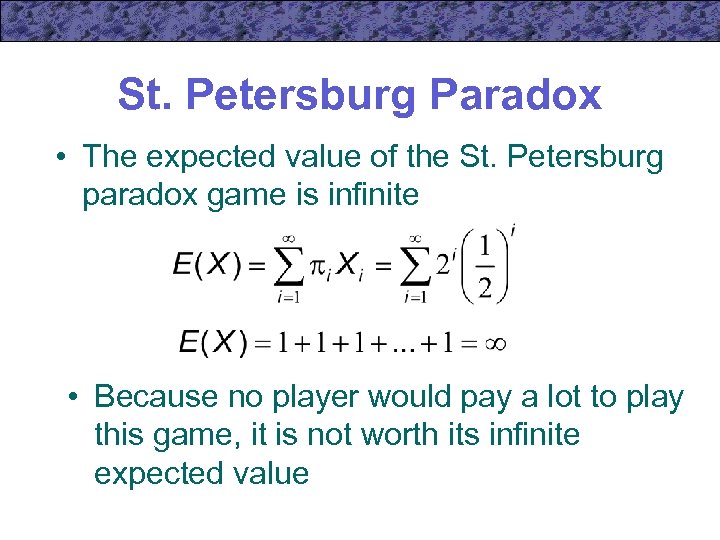St. Petersburg Paradox • The expected value of the St. Petersburg paradox game is infinite • Because no player would pay a lot to play this game, it is not worth its infinite expected value

Expected Utility • Individuals do not care directly about the dollar values of the prizes – they care about the utility that the dollars provide • If we assume diminishing marginal utility of income, the St. Petersburg game may converge to a finite expected utility value – this would measure how much the game is worth to the individual

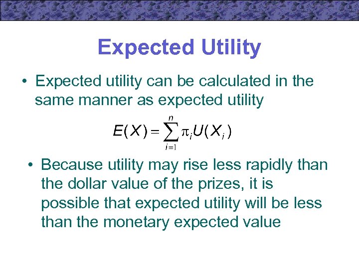Expected Utility • Expected utility can be calculated in the same manner as expected utility • Because utility may rise less rapidly than the dollar value of the prizes, it is possible that expected utility will be less than the monetary expected value

The Von Neumann. Morgenstern Theorem • Suppose that there are n possible prizes that an individual might win (X 1, …Xn) arranged in ascending order of desirability – X 1 = least preferred prize = 0 – Xn = most preferred prize = 1

The Von Neumann. Morgenstern Theorem • The point of the von Neumann. Morgenstern theorem is to show that there is a reasonable way to assign specific utility numbers to the other prizes available

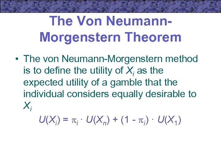The Von Neumann. Morgenstern Theorem • The von Neumann-Morgenstern method is to define the utility of Xi as the expected utility of a gamble that the individual considers equally desirable to Xi U(Xi) = i · U(Xn) + (1 - i) · U(X 1)

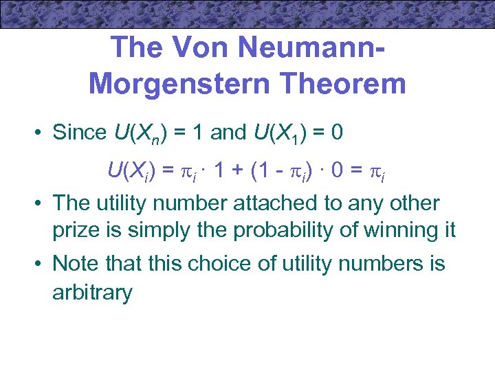The Von Neumann. Morgenstern Theorem • Since U(Xn) = 1 and U(X 1) = 0 U(Xi) = i · 1 + (1 - i) · 0 = i • The utility number attached to any other prize is simply the probability of winning it • Note that this choice of utility numbers is arbitrary

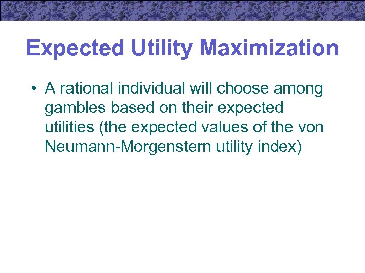Expected Utility Maximization • A rational individual will choose among gambles based on their expected utilities (the expected values of the von Neumann-Morgenstern utility index)

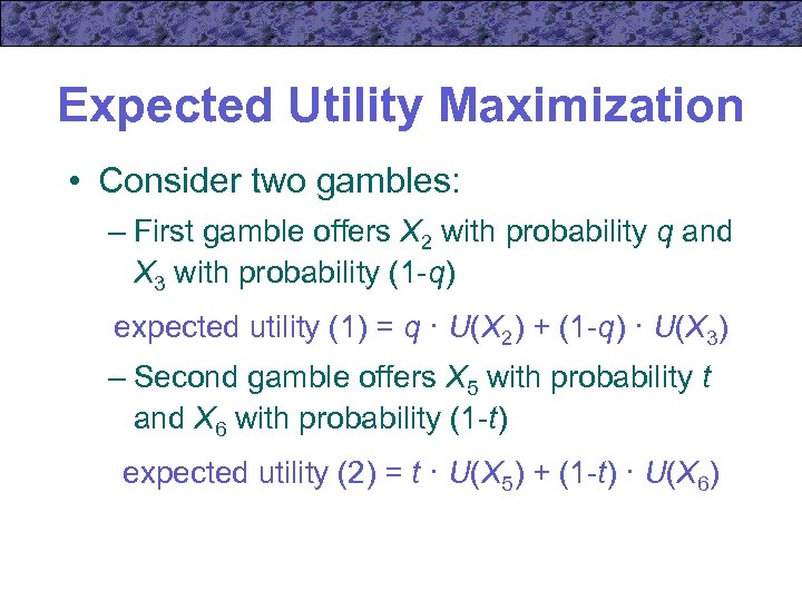Expected Utility Maximization • Consider two gambles: – First gamble offers X 2 with probability q and X 3 with probability (1 -q) expected utility (1) = q · U(X 2) + (1 -q) · U(X 3) – Second gamble offers X 5 with probability t and X 6 with probability (1 -t) expected utility (2) = t · U(X 5) + (1 -t) · U(X 6)

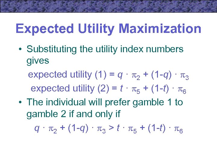Expected Utility Maximization • Substituting the utility index numbers gives expected utility (1) = q · 2 + (1 -q) · 3 expected utility (2) = t · 5 + (1 -t) · 6 • The individual will prefer gamble 1 to gamble 2 if and only if q · 2 + (1 -q) · 3 > t · 5 + (1 -t) · 6

Expected Utility Maximization • If individuals obey the von Neumann. Morgenstern axioms of behavior in uncertain situations, they will act as if they choose the option that maximizes the expected value of their von Neumann-Morgenstern utility index

Risk Aversion • Two games may have the same expected value but differ in their riskiness – Flip a coin for $1 versus $1, 000 • Risk refers to the variability of the outcomes of some uncertain activity • When faced with two gambles of the same expected value, individuals will usually choose the one with lower risk

Risk Aversion • In general, we assume that the marginal utility of prize money falls as the prize gets larger – A flip of a coin for $1, 000 promises a small gain in utility if you win, but a large loss in utility if you lose – A flip of a coin for $1 is inconsequential as the gain in utility from a win is not much different as the drop in utility from a loss

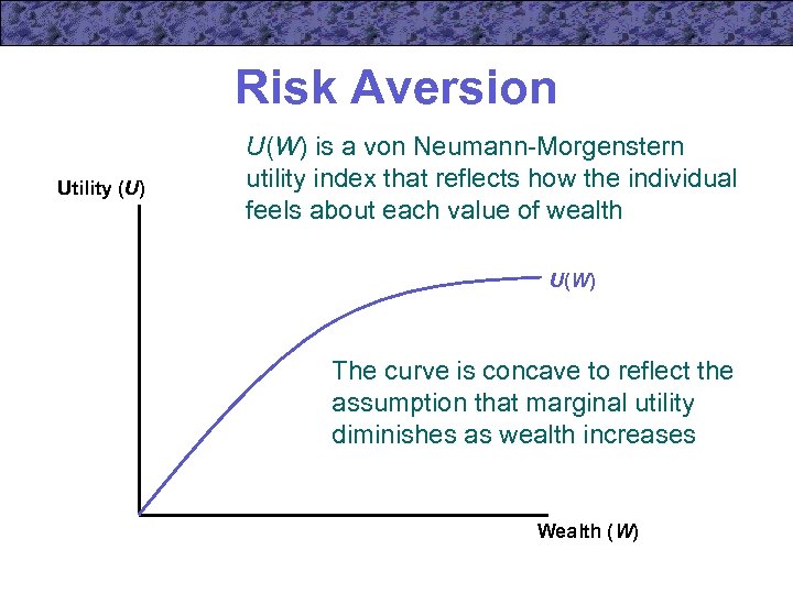Risk Aversion Utility (U) U(W) is a von Neumann-Morgenstern utility index that reflects how the individual feels about each value of wealth U(W) The curve is concave to reflect the assumption that marginal utility diminishes as wealth increases Wealth (W)

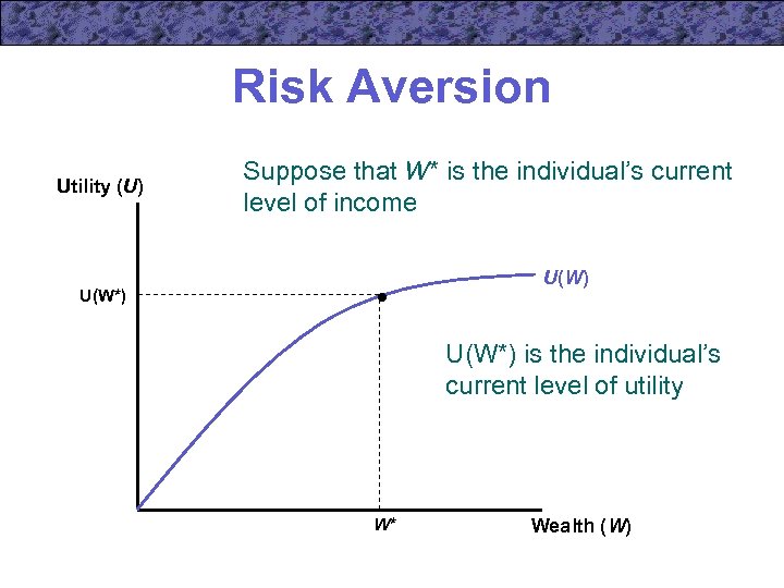Risk Aversion Utility (U) Suppose that W* is the individual’s current level of income U(W) U(W*) is the individual’s current level of utility W* Wealth (W)

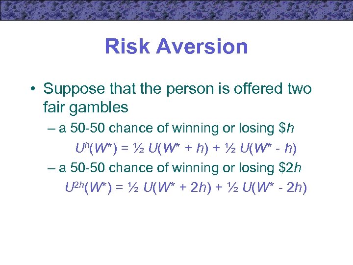Risk Aversion • Suppose that the person is offered two fair gambles – a 50 -50 chance of winning or losing $h Uh(W*) = ½ U(W* + h) + ½ U(W* - h) – a 50 -50 chance of winning or losing $2 h U 2 h(W*) = ½ U(W* + 2 h) + ½ U(W* - 2 h)

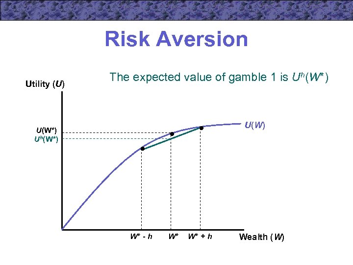Risk Aversion Utility (U) The expected value of gamble 1 is Uh(W*) U(W*) Uh(W*) W* - h W* W* + h Wealth (W)

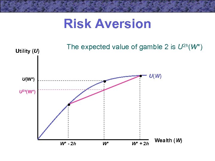Risk Aversion Utility (U) The expected value of gamble 2 is U 2 h(W*) U(W*) U 2 h(W*) W* - 2 h W* W* + 2 h Wealth (W)

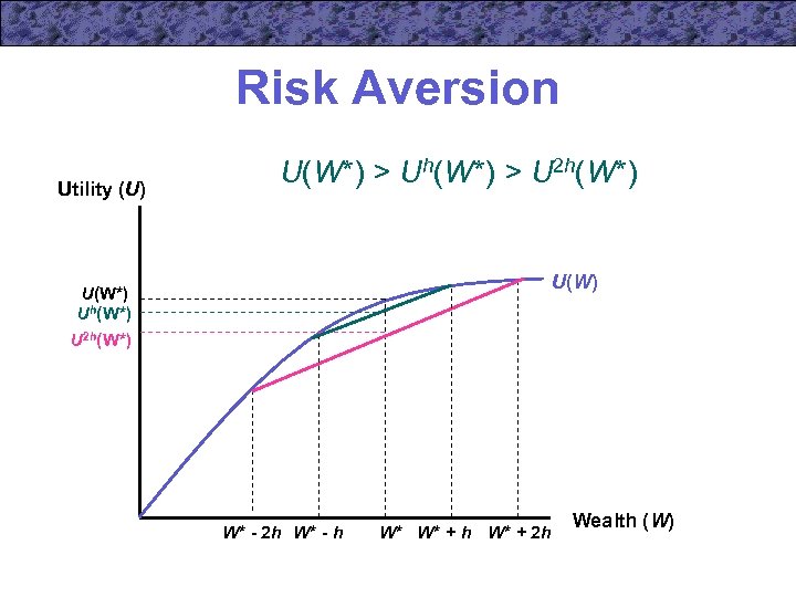Risk Aversion Utility (U) U(W*) > Uh(W*) > U 2 h(W*) U(W*) Uh(W*) U 2 h(W*) W* - 2 h W* - h W* W* + h W* + 2 h Wealth (W)

Risk Aversion • The person will prefer current wealth to that wealth combined with a fair gamble • The individual will also prefer a small gamble over a large one

Risk Aversion and Insurance • The person might be willing to pay some amount to avoid participating in a gamble • This helps to explain why some individuals purchase insurance

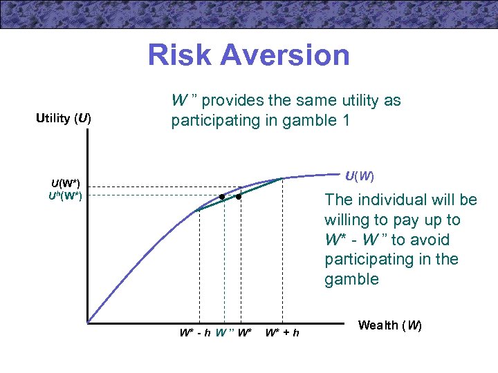Risk Aversion Utility (U) W ” provides the same utility as participating in gamble 1 U(W) U(W*) Uh(W*) The individual will be willing to pay up to W* - W ” to avoid participating in the gamble W* - h W ” W* W* + h Wealth (W)

Risk Aversion • An individual who always refuses fair bets is said to be risk averse – will exhibit diminishing marginal utility of income – will be willing to pay to avoid taking fair bets

Risk Aversion and Insurance • Consider a person with a current wealth of $100, 000 who faces a 25% chance of losing his automobile worth $20, 000 • Suppose also that the person’s von Neumann-Morgenstern utility index is U(W) = ln (W)

Risk Aversion and Insurance • The person’s expected utility will be E(U) = 0. 75 U(100, 000) + 0. 25 U(80, 000) E(U) = 0. 75 ln(100, 000) + 0. 25 ln(80, 000) E(U) = 11. 45714 • Note that a fair insurance premium would be $5, 000 (25% of $20, 000)

Risk Aversion and Insurance • The individual will likely be willing to pay more than $5, 000 to avoid the gamble. How much will he pay? E(U) = U(100, 000 - x) = ln(100, 000 - x) = 11. 45714 100, 000 - x = e 11. 45714 x = 5, 426 • The maximum premium is $5, 426

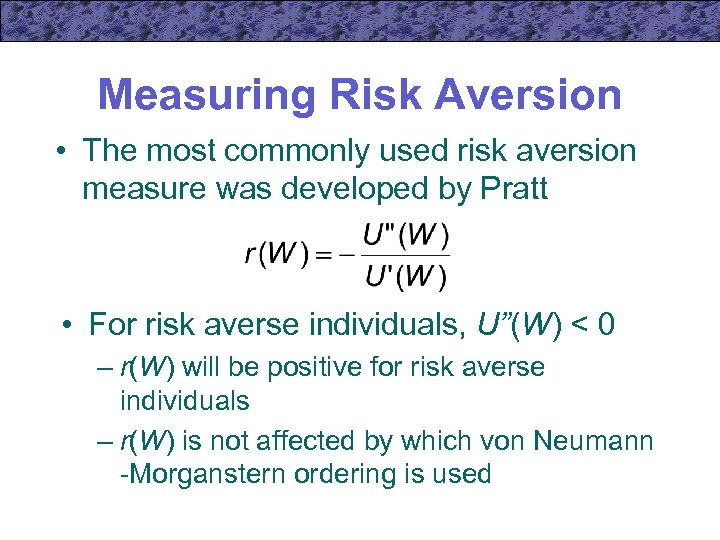Measuring Risk Aversion • The most commonly used risk aversion measure was developed by Pratt • For risk averse individuals, U”(W) < 0 – r(W) will be positive for risk averse individuals – r(W) is not affected by which von Neumann -Morganstern ordering is used

Measuring Risk Aversion • The Pratt risk aversion measure is proportional to the amount an individual will pay to avoid a fair gamble

Measuring Risk Aversion • Let h be the winnings from a fair bet E(h) = 0 • Let p be the size of the insurance premium that would make the individual exactly indifferent between taking the fair bet h and paying p with certainty to avoid the gamble E[U(W + h)] = U(W - p)

Measuring Risk Aversion • We now need to expand both sides of the equation using Taylor’s series • Because p is a fixed amount, we can use a simple linear approximiation to the right-hand side U(W - p) = U(W) - p. U’(W) + higher order terms

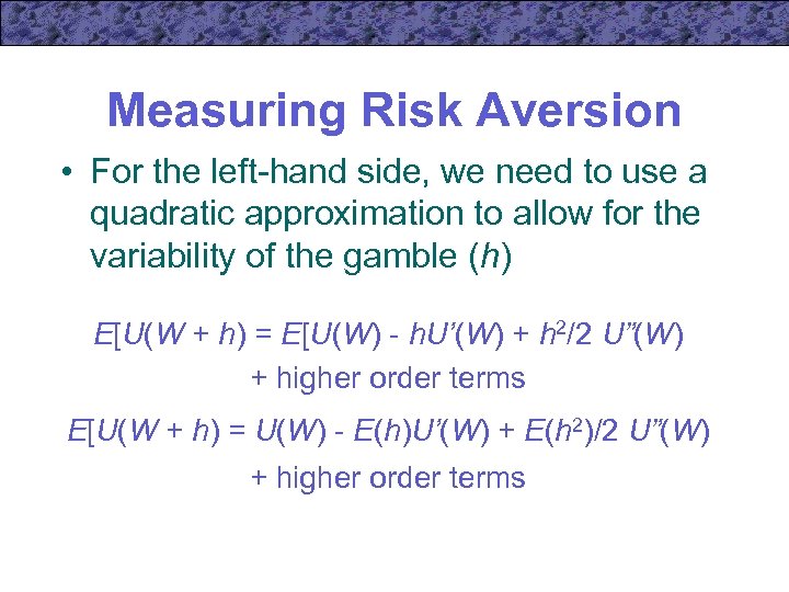Measuring Risk Aversion • For the left-hand side, we need to use a quadratic approximation to allow for the variability of the gamble (h) E[U(W + h) = E[U(W) - h. U’(W) + h 2/2 U”(W) + higher order terms E[U(W + h) = U(W) - E(h)U’(W) + E(h 2)/2 U”(W) + higher order terms

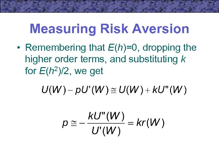Measuring Risk Aversion • Remembering that E(h)=0, dropping the higher order terms, and substituting k for E(h 2)/2, we get

Risk Aversion and Wealth • It is not necessarily true that risk aversion declines as wealth increases – diminishing marginal utility would make potential losses less serious for high-wealth individuals – however, diminishing marginal utility also makes the gains from winning gambles less attractive – The net result depends on the shape of the utility function

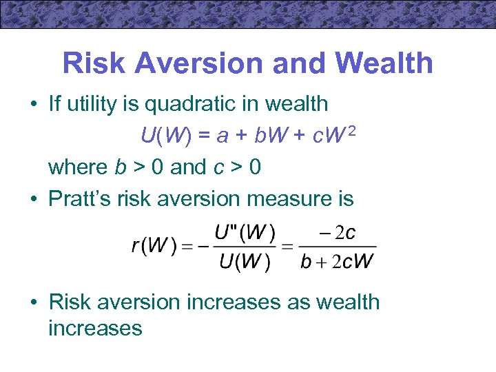Risk Aversion and Wealth • If utility is quadratic in wealth U(W) = a + b. W + c. W 2 where b > 0 and c > 0 • Pratt’s risk aversion measure is • Risk aversion increases as wealth increases

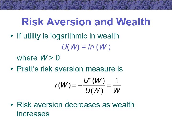Risk Aversion and Wealth • If utility is logarithmic in wealth U(W) = ln (W ) where W > 0 • Pratt’s risk aversion measure is • Risk aversion decreases as wealth increases

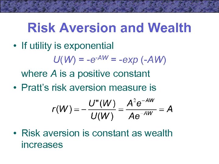Risk Aversion and Wealth • If utility is exponential U(W) = -e-AW = -exp (-AW) where A is a positive constant • Pratt’s risk aversion measure is • Risk aversion is constant as wealth increases

Relative Risk Aversion • It seems unlikely that the willingness to pay to avoid a gamble is independent of wealth • A more appealing assumption may be that the willingness to pay is inversely proportional to wealth

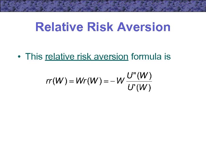Relative Risk Aversion • This relative risk aversion formula is

The State-Preference Approach • The approach taken in this chapter up to this point is different from the approach taken in other chapters – has not used the basic model of utilitymaximization subject to a budget constraint • There is a need to develop new techniques to incorporate the standard choice-theoretic framework

States of the World • Outcomes of any random event can be categorized into a number of states of the world – “good times” or “bad times” • Contingent commodities are goods delivered only if a particular state of the world occurs – “$1 in good times” or “$1 in bad times”

States of the World • It is conceivable that an individual could purchase a contingent commodity – buy a promise that someone will pay you $1 if tomorrow turns out to be good times – this good will probably cost less than $1

Utility Analysis • Assume that there are two contingent goods – wealth in good times (Wg) and wealth in bad times (Wb) – individual believes the probability of good times is

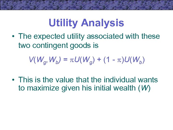Utility Analysis • The expected utility associated with these two contingent goods is V(Wg, Wb) = U(Wg) + (1 - )U(Wb) • This is the value that the individual wants to maximize given his initial wealth (W)

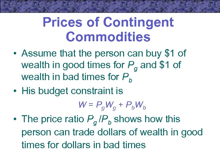Prices of Contingent Commodities • Assume that the person can buy $1 of wealth in good times for Pg and $1 of wealth in bad times for Pb • His budget constraint is W = P g. W g + P b. W b • The price ratio Pg /Pb shows how this person can trade dollars of wealth in good times for dollars in bad times

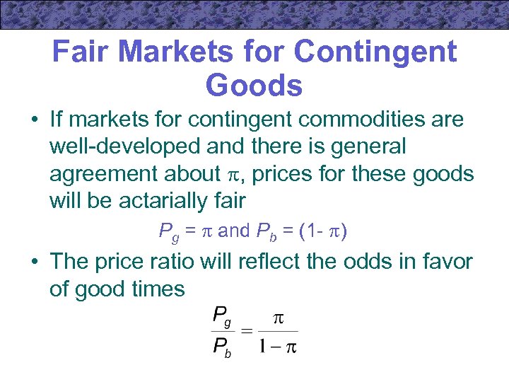Fair Markets for Contingent Goods • If markets for contingent commodities are well-developed and there is general agreement about , prices for these goods will be actarially fair Pg = and Pb = (1 - ) • The price ratio will reflect the odds in favor of good times

Risk Aversion • If contingent claims markets are fair, a utility-maximizing individual will opt for a situation in which Wg = Wb – he will arrange matters so that the wealth obtained is the same no matter what state occurs

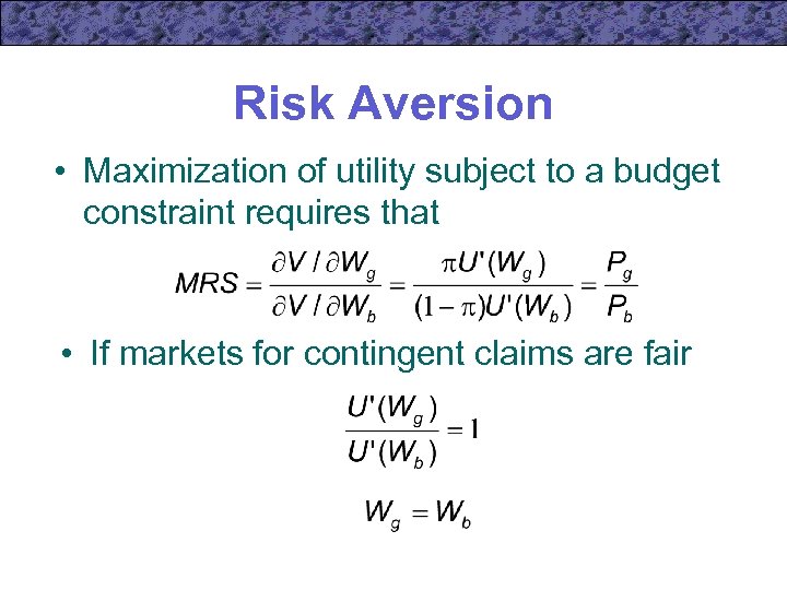Risk Aversion • Maximization of utility subject to a budget constraint requires that • If markets for contingent claims are fair

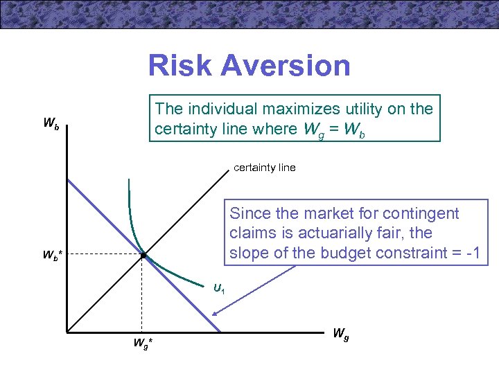Risk Aversion The individual maximizes utility on the certainty line where Wg = Wb Wb certainty line Since the market for contingent claims is actuarially fair, the slope of the budget constraint = -1 Wb * U 1 Wg * Wg

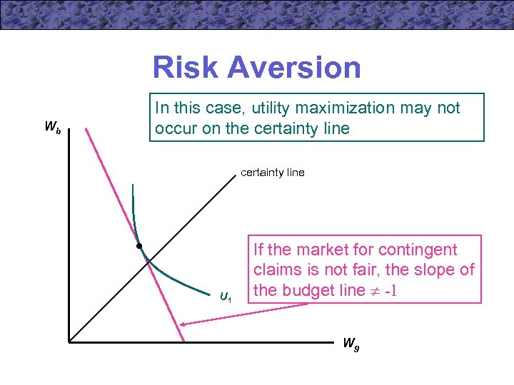Risk Aversion Wb In this case, utility maximization may not occur on the certainty line U 1 If the market for contingent claims is not fair, the slope of the budget line -1 Wg

Insurance in the State. Preference Model • Again, consider a person with wealth of $100, 000 who faces a 25% chance of losing his automobile worth $20, 000 – Wealth with no theft (Wg) = $100, 000 and probability of no theft = 0. 75 – Wealth with a theft (Wb) = $80, 000 and probability of a theft = 0. 25

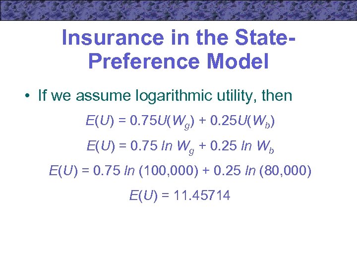Insurance in the State. Preference Model • If we assume logarithmic utility, then E(U) = 0. 75 U(Wg) + 0. 25 U(Wb) E(U) = 0. 75 ln Wg + 0. 25 ln Wb E(U) = 0. 75 ln (100, 000) + 0. 25 ln (80, 000) E(U) = 11. 45714

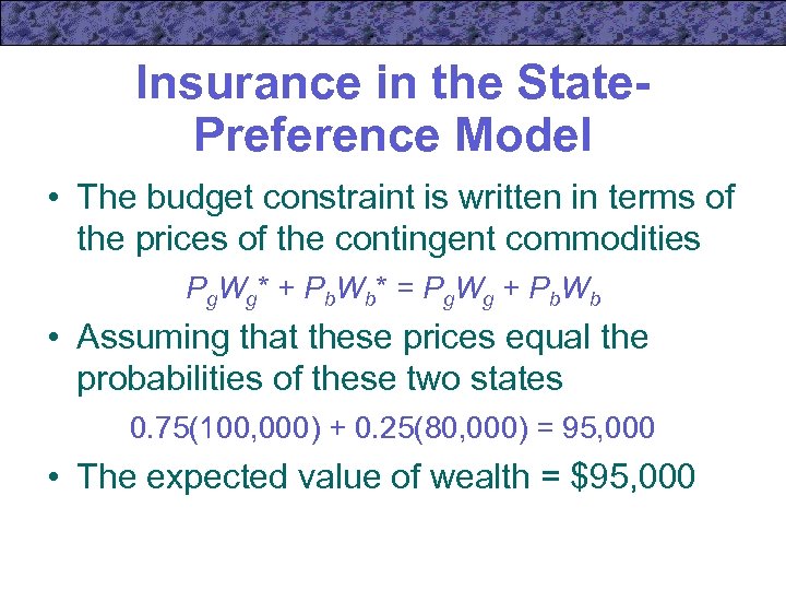Insurance in the State. Preference Model • The budget constraint is written in terms of the prices of the contingent commodities P g. W g* + P b. W b* = P g. W g + P b. W b • Assuming that these prices equal the probabilities of these two states 0. 75(100, 000) + 0. 25(80, 000) = 95, 000 • The expected value of wealth = $95, 000

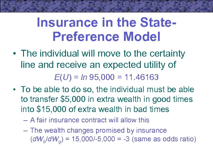Insurance in the State. Preference Model • The individual will move to the certainty line and receive an expected utility of E(U) = ln 95, 000 = 11. 46163 • To be able to do so, the individual must be able to transfer $5, 000 in extra wealth in good times into $15, 000 of extra wealth in bad times – A fair insurance contract will allow this – The wealth changes promised by insurance (d. Wb/d. Wg) = 15, 000/-5, 000 = -3 (same as odds ratio)

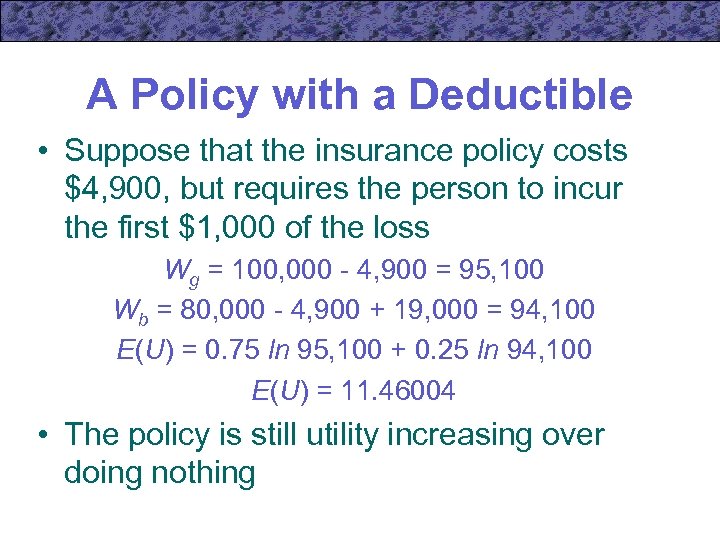A Policy with a Deductible • Suppose that the insurance policy costs $4, 900, but requires the person to incur the first $1, 000 of the loss Wg = 100, 000 - 4, 900 = 95, 100 Wb = 80, 000 - 4, 900 + 19, 000 = 94, 100 E(U) = 0. 75 ln 95, 100 + 0. 25 ln 94, 100 E(U) = 11. 46004 • The policy is still utility increasing over doing nothing

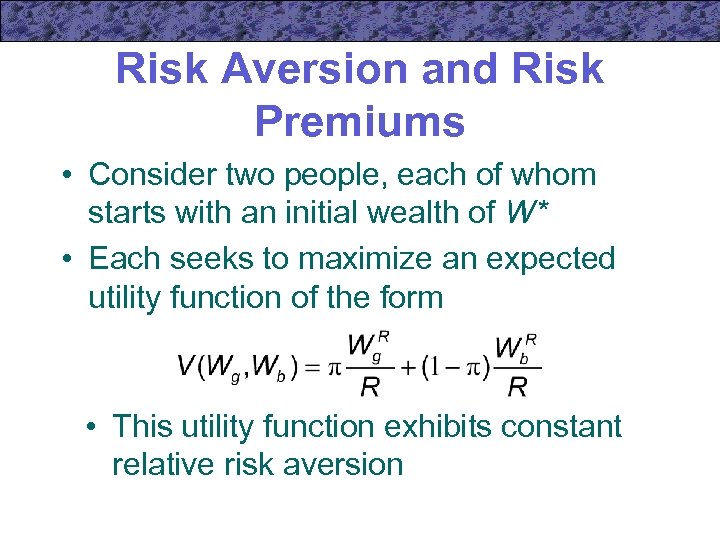Risk Aversion and Risk Premiums • Consider two people, each of whom starts with an initial wealth of W* • Each seeks to maximize an expected utility function of the form • This utility function exhibits constant relative risk aversion

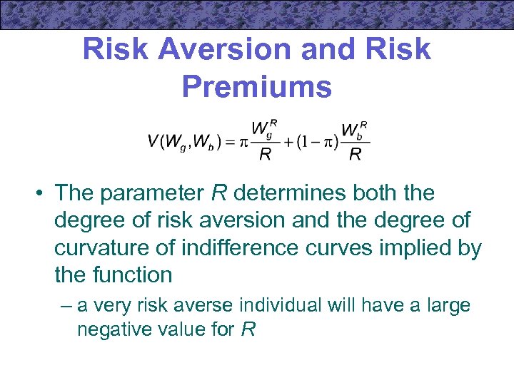Risk Aversion and Risk Premiums • The parameter R determines both the degree of risk aversion and the degree of curvature of indifference curves implied by the function – a very risk averse individual will have a large negative value for R

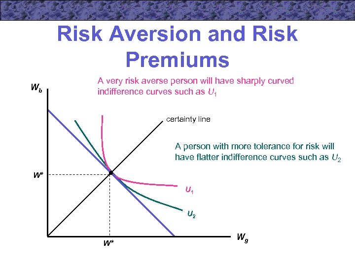Risk Aversion and Risk Premiums Wb A very risk averse person will have sharply curved indifference curves such as U 1 certainty line A person with more tolerance for risk will have flatter indifference curves such as U 2 W* U 1 U 2 W* Wg

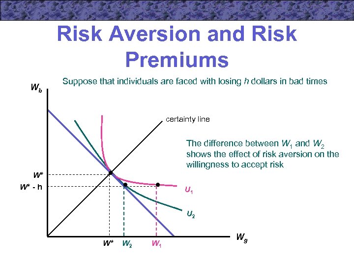Risk Aversion and Risk Premiums Wb Suppose that individuals are faced with losing h dollars in bad times certainty line The difference between W 1 and W 2 shows the effect of risk aversion on the willingness to accept risk W* W* - h U 1 U 2 W* W 2 W 1 Wg

Important Points to Note: • In uncertain situations, individuals are concerned with the expected utility of various outcomes – if they obey the von Neumann-Morgenstern axioms, they will make choices that maximize expected utility • If we assume that individuals exhibit a diminishing marginal utility of income, they will also be risk averse – they will refuse to take actuarially fair bets

Important Points to Note: • Risk averse individuals will wish to insure themselves completely against uncertain events if premiums are actarially fair – may be willing to pay actuarially unfair premiums to avoid taking risks

Important Points to Note: • Decisions under uncertainty can be analyzed in a choice-theoretic framework by using the state-preference approach among contingent commodities – if preferences are state-independent and prices are actuarially fair, individuals will prefer allocations along the “certainty line” • will receive the same level of wealth regardless of which state occurs