ea666647937761db04951b2c0dd41073.ppt
- Количество слайдов: 116
Chapter 7 The Firm
Business Firm • Employs factors of production • Produces goods and services • Sells to consumers, other firms, or the government • We work for and buy from firms
Market • Two sides – Buyers • Utility is major decision making device – Sellers • How do they make decisions
How do the two sides come together? • Market Coordination – Invisible Hand (Adam Smith) – Market guides individuals into activities at which they are the most efficient – Pushes sellers to produce certain things and buyers to instruct what to produce – Equates supply and demand
How does the firm decide what to produce? • Managerial Coordination – Guides individual firm production decisions – Thus…invisible hand of the firm
Why follow this invisible hand? • Firms are formed because greater benefits of working as a team than working as individuals
Problem with teamwork • Shirking – Putting forth less effort than your originally agreed to – Problem because shirker gains ALL benefits from shirking but costs are spread over the entire team
Can shirking increase or decrease? • Yes!! • As the benefits of shirking increase so does the amount • If the shirker must bear the full cost of shirking then shirking will decrease
How can we decrease shirking? • Manager’s duty or MONITORING • Reward productive workers and punish shirkers • Preserves the benefit of team production • Reduces the benefits of shirking
Who monitors the monitor? • Salary usually tied into production • Called Residual Claimant – Person who shares in the profits of the firm – More shirkers? ? Less Production…so less pay for monitor
Another way to ward off shirking? • Pay higher than equilibrium wages • Decreases shirking because cost of losing job is greater. • Don’t need monitor because high wage makes worker monitor themselves • Called efficiency wage theory
Why do people submit to being monitored? ? • Monitoring decreases shirking • Monitoring increases benefits of teamwork • Monitoring maximizes benefits that can be achieved
Objective of the firm • Profit Maximization • Now…want to move to the Firm to see how they achieve this objective
Chapter 8 Production and Costs © South-Western College Publishing 1998
Cost Side • Explicit Cost – Actual money is exchanged – COST • Implicit Cost – Value of resources used in the production or acquisition of a good – No monetary payment – OPPORTUNITY COST
Sacrifice • In order to have a cost, sacrifice must have taken place • Forfeited something else • No money must change hands for sacrifice to take place
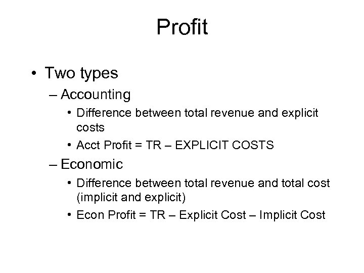
Profit • Two types – Accounting • Difference between total revenue and explicit costs • Acct Profit = TR – EXPLICIT COSTS – Economic • Difference between total revenue and total cost (implicit and explicit) • Econ Profit = TR – Explicit Cost – Implicit Cost
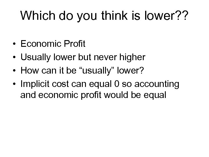
Which do you think is lower? ? • • Economic Profit Usually lower but never higher How can it be “usually” lower? Implicit cost can equal 0 so accounting and economic profit would be equal
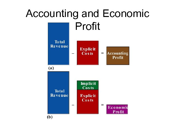
Accounting and Economic Profit
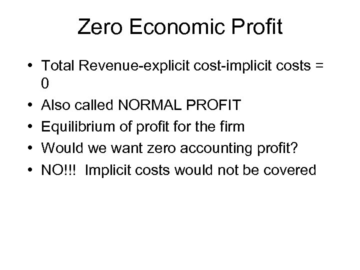
Zero Economic Profit • Total Revenue-explicit cost-implicit costs = 0 • Also called NORMAL PROFIT • Equilibrium of profit for the firm • Would we want zero accounting profit? • NO!!! Implicit costs would not be covered
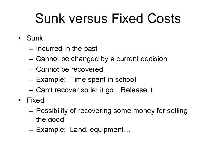
Sunk versus Fixed Costs • Sunk – Incurred in the past – Cannot be changed by a current decision – Cannot be recovered – Example: Time spent in school – Can’t recover so let it go…Release it • Fixed – Possibility of recovering some money for selling the good – Example: Land, equipment…
Production • Takes time to produce • Costly to produce • Direct link between production, costs, and time
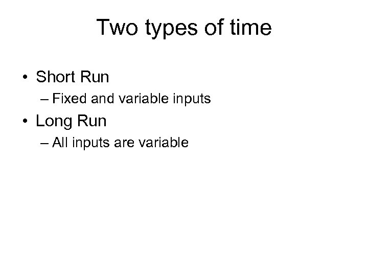
Two types of time • Short Run – Fixed and variable inputs • Long Run – All inputs are variable
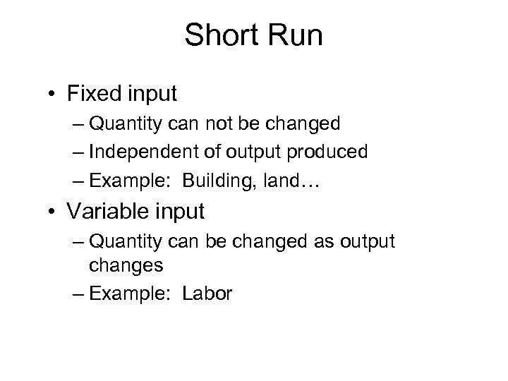
Short Run • Fixed input – Quantity can not be changed – Independent of output produced – Example: Building, land… • Variable input – Quantity can be changed as output changes – Example: Labor
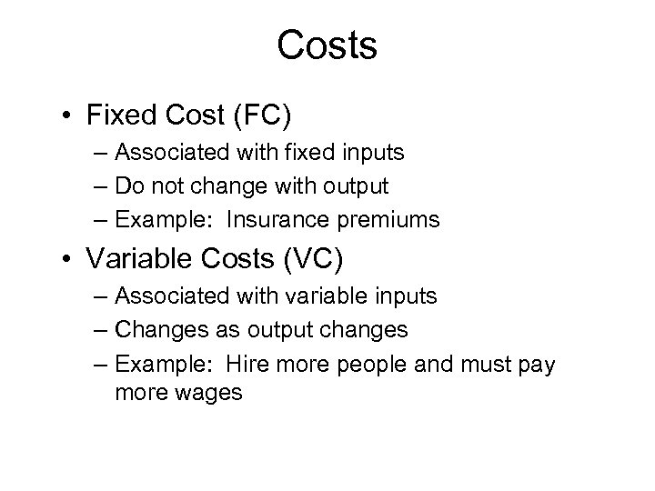
Costs • Fixed Cost (FC) – Associated with fixed inputs – Do not change with output – Example: Insurance premiums • Variable Costs (VC) – Associated with variable inputs – Changes as output changes – Example: Hire more people and must pay more wages
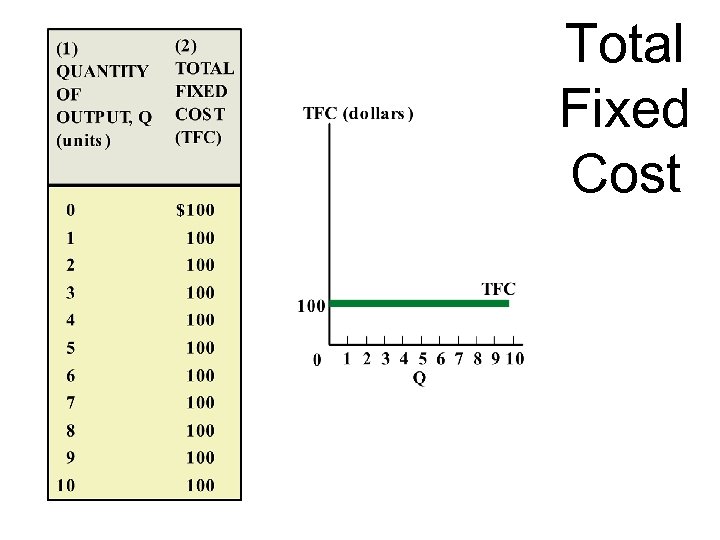
Total Fixed Cost
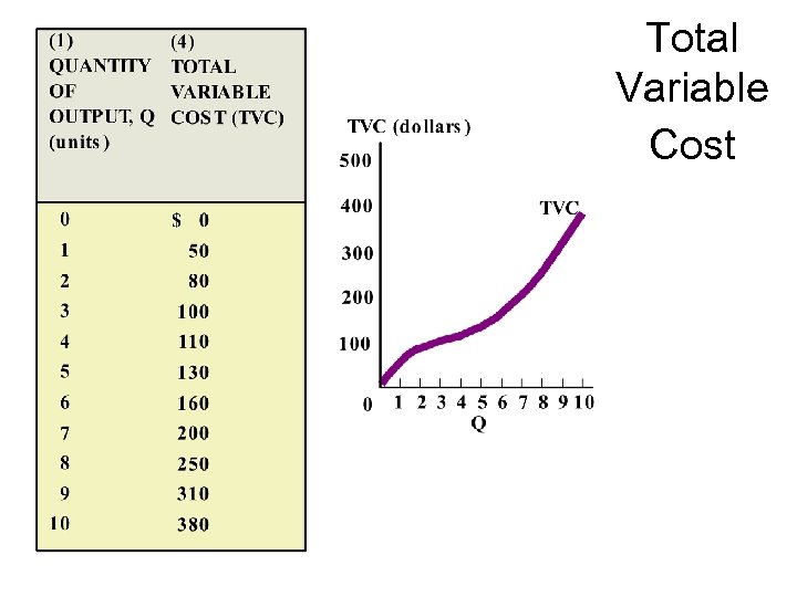
Total Variable Cost
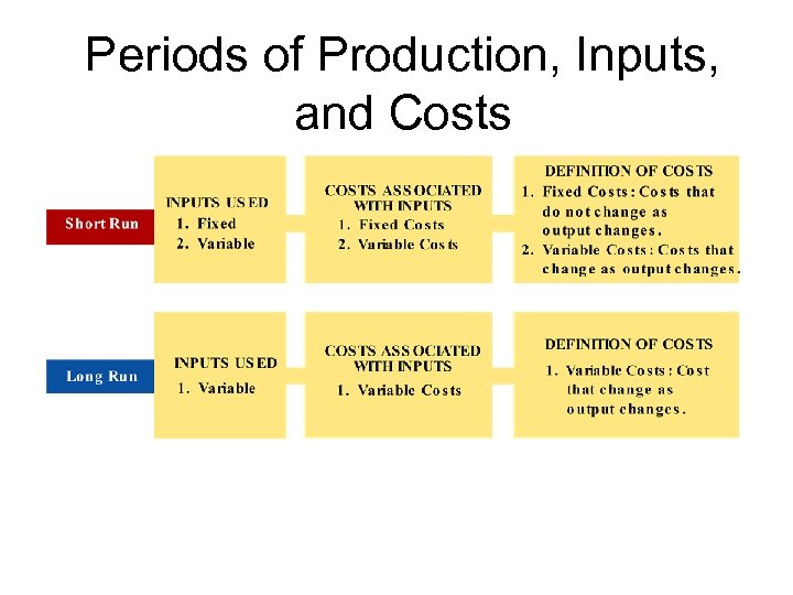
Periods of Production, Inputs, and Costs
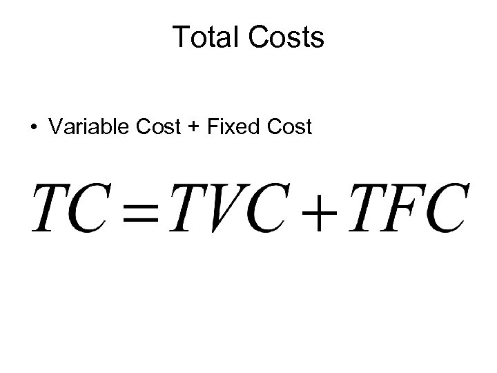
Total Costs • Variable Cost + Fixed Cost
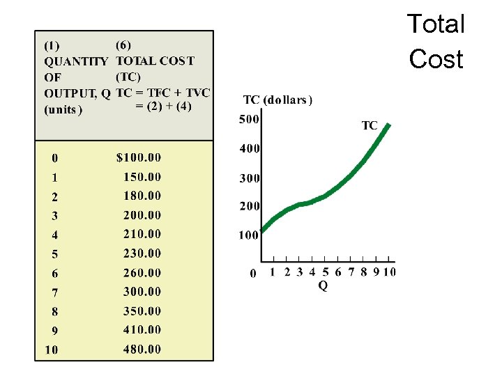
Total Cost
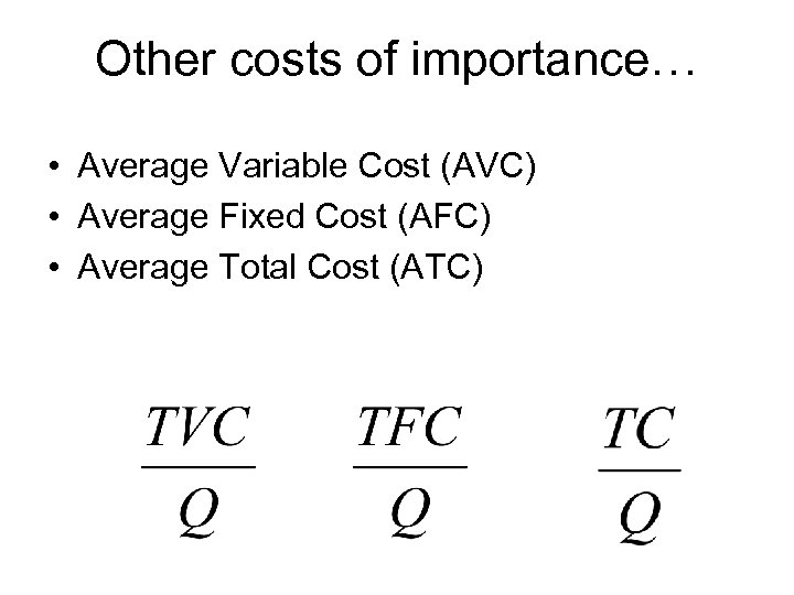
Other costs of importance… • Average Variable Cost (AVC) • Average Fixed Cost (AFC) • Average Total Cost (ATC)
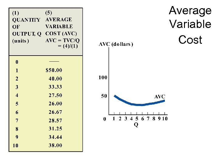
Average Variable Cost
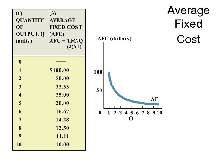
Average Fixed Cost
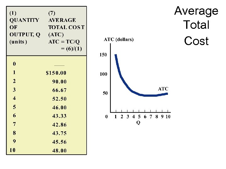
Average Total Cost
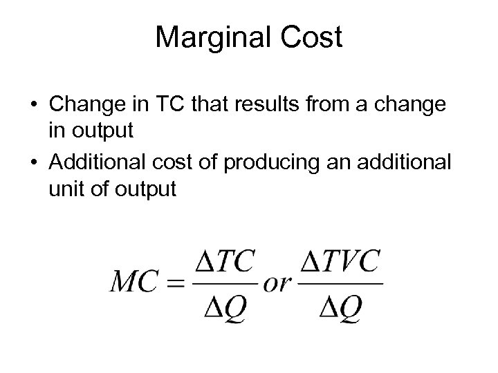
Marginal Cost • Change in TC that results from a change in output • Additional cost of producing an additional unit of output
Why Change in Total Cost or Total Variable Cost? ? • Since total fixed cost doesn’t change the “additional” total fixed cost is zero
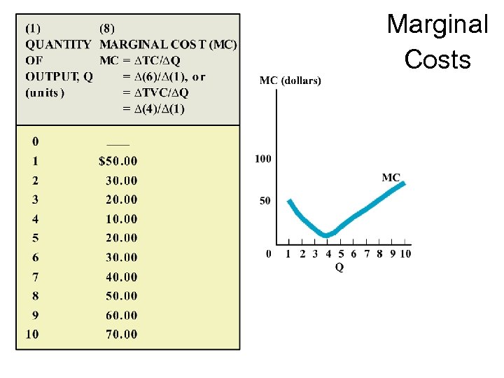
Marginal Costs

In-class exercise #9 Using the knowledge
Shapes of Curves • Law of diminishing marginal returns – As larger amounts of a variable input are combined with fixed inputs eventually the Marginal Physical Product (MPP) declines
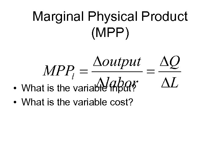
Marginal Physical Product (MPP) • What is the variable input? • What is the variable cost?
So… • As more labor (VARIABLE INPUT) are added to land (FIXED INPUT) the variable inputs would yield smaller and smaller additions to output
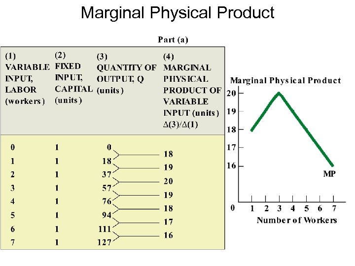
Marginal Physical Product
Crowding Problem • The point at which MPP declines • Shows the law of diminishing returns
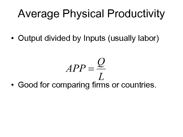
Average Physical Productivity • Output divided by Inputs (usually labor) • Good for comparing firms or countries.
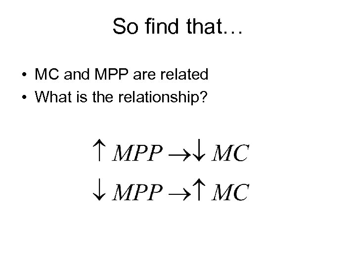
So find that… • MC and MPP are related • What is the relationship?

0 ing 1 h e is is in rc im e ex D ? s ow ? as sh s? cl – P urn In MP et R s e o D
Law of Diminishing Marginal Returns
Marginal Cost
Does this relationship make sense? • Yes. . • If productivity increases what would happen to costs? ? – Decrease (MPP increase & MC decrease) • Productivity decreases? ? – Increase (MPP decreases & MC increases)
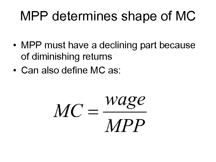
MPP determines shape of MC • MPP must have a declining part because of diminishing returns • Can also define MC as:
In-class exercise 11 How do we calculate these costs? ? Give two ways to get to the cost…
Average-Marginal Rule • Can use to see what the ATC and AVC curve look like • Tells us what happens when MC is above or below the “average” curves • If MC is above AVC and ATC – AVC and ATC are rising • If MC is below AVC and ATC – AVC and ATC are falling
From Average-Marginal Rule can infer… • MC intersects the AVC and ATC curves at their MINIMUM POINTS • Cannot infer anything about AFC
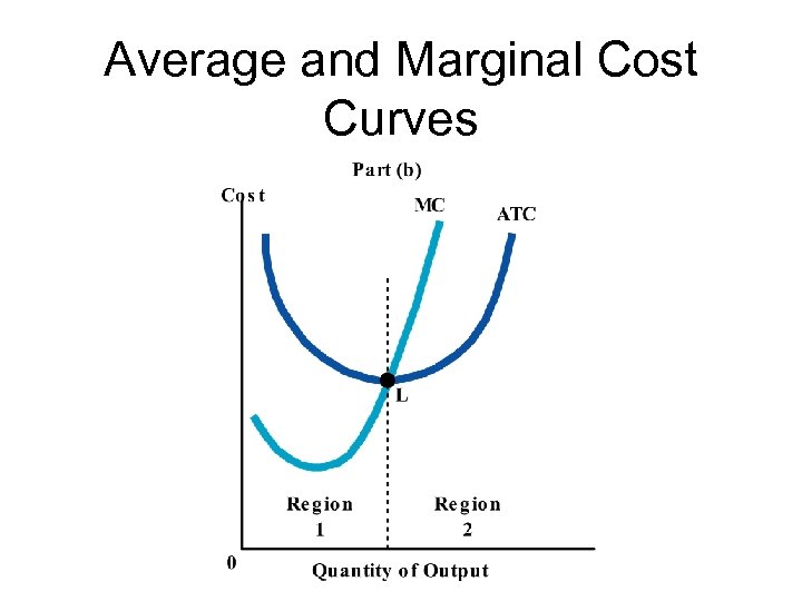
Average and Marginal Cost Curves
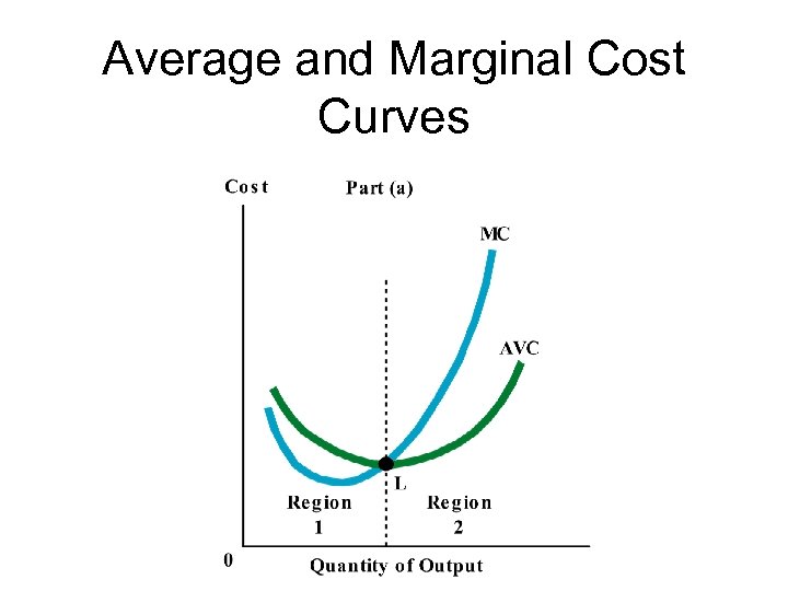
Average and Marginal Cost Curves
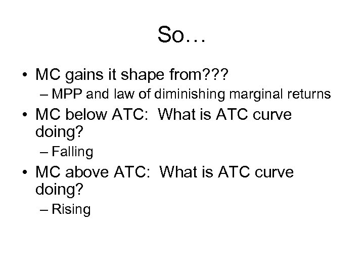
So… • MC gains it shape from? ? ? – MPP and law of diminishing marginal returns • MC below ATC: What is ATC curve doing? – Falling • MC above ATC: What is ATC curve doing? – Rising
Average and Marginal Cost Curves
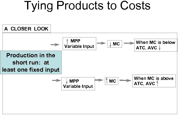
Tying Products to Costs A CLOSER LOOK MPP Variable Input MC When MC is below ATC, AVC Production in the short run: at least one fixed input MPP Variable Input MC When MC is above ATC, AVC
Now switching to the Long Run • When does Long Run start? – As soon as all inputs (costs) are VARIABLE – No fixed costs • Important curves – LRTC – LRATC – LRMC
Short Run vs. Long Run • Short Run assumes FIXED plant size • Each plant size has a unique ATC curve associated with it – SRATC • LRATC combines all the SRATC curves • Which points of the SRATC? ? ? • Minimum points
Why minimum? • LRATC shows the lowest average cost at which a firm can produce any given level of output • LRATC is the lower ENVELOPE of the SRATC curves • Called envelope curve
Long-Run Average Total Cost Curve (LRATC)
Isn’t the LRATC curve smooth? ? • Yes!! • Have infinitely many SRATC curves so it would be smooth if use all curves • Each SRATC curve touches the LRATC curve only once
Shape of LRATC • U-shaped • Decreasing, Flat, then Increasing • Important when finding optimal long run output level
Long-Run Average Total Cost Curve (LRATC)
Economies of Scale • Downward part of LRATC • Average costs decrease as output increases • If have a 1% increase in input usage what happens to output? ? – Increases by MORE than 1% • Specialization
Constant Returns to Scale • Flat portion of LRATC • Costs remain the same as increase output • If have a 1% increase in input usage what happens to output? ? – Output increases by EXACTLY 1% • First point of constant returns to scale is called MINIMUM EFFICIENT SCALE
Diseconomies of Scale • Upward sloped portion of LRATC • Costs are rising as we increase output • If have a 1% increase in input usage what happens to output? – Increases by LESS THAN 1% • Why? ? ? – Firm too large (bad communication or coordination problems)
Long-Run Average Total Cost Curve (LRATC)
Are economies, diseconomies, and constant returns to scale in SR, LR, or both? ? ? • LONG RUN ONLY!!! • Why? – Inputs necessary for production are able to be changed – No fixed inputs
Is this the same as diminishing returns? • NO • Diminishing returns is from using ONE plant size intensely – Short run • Economies of scale is from CHANGING plant size – Long run
Review • Economies of Scale – LRATC falling • Constant Returns to Scale – LRATC flat • Diseconomies of Scale – LRATC rising
Why does economies of scale exist? • Large firms offer more opportunity for workers to specialize • Growing firms can take advantage of efficient mass production techniques – Smooth cost over more units produced
Why does diseconomies of scale exist? • Communication problems • Shirking • Management problems
Why is minimum efficient scale important? • Lowest output level at which ATC are minimized • Which has a cost advantage? ? – Small firm at minimum efficient scale point – Larger firm producing more output but still within constant returns to scale area – Neither
Long-Run Average Total Cost Curve (LRATC)
Minimum Efficient Scale for Six Industries
Where would you expect to find less firms? (using MES) • Firms with higher MES • Why? ? – Produce until MES – If MES is higher then each firm will be producing more…so need less firms to cover quantity wanted by economy • Many SHOE companies (MES =. 2) • Few REFRIGERATOR companies (MES = 14)
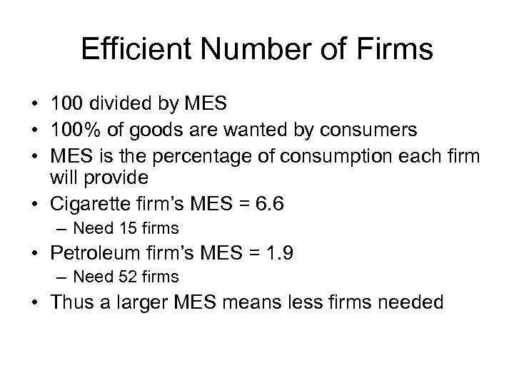
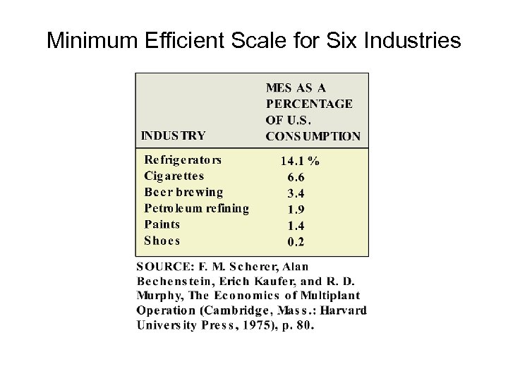
Efficient Number of Firms • 100 divided by MES • 100% of goods are wanted by consumers • MES is the percentage of consumption each firm will provide • Cigarette firm’s MES = 6. 6 – Need 15 firms • Petroleum firm’s MES = 1. 9 – Need 52 firms • Thus a larger MES means less firms needed
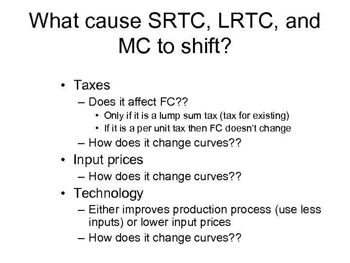
What cause SRTC, LRTC, and MC to shift? • Taxes – Does it affect FC? ? • Only if it is a lump sum tax (tax for existing) • If it is a per unit tax then FC doesn’t change – How does it change curves? ? • Input prices – How does it change curves? ? • Technology – Either improves production process (use less inputs) or lower input prices – How does it change curves? ?

Homework due Monday May 19 th • Chapter 8 – Questions: 3, 5, 10, and 11 • Working with numbers and graphs – Questions 3, 6, and 7
In-class exercise 12 Do we understand Chapter 8? ?
Chapter 10 MONOPOLY
Assumptions • One seller – Firm is the industry • No substitutes for good • Many barriers to entry
Government can “grant” monopoly power in three ways… • Public franchise – Exclusive provider • Power companies, water companies • Patents – Exclusive provider for 17 years – Encourages people to invent new things • Zantac, Tagament • Licenses – Must have to operate • Cabs in New York City
Monopolies exist because: • Legal mandate – Government allows or doesn’t allow you to operate • Economic rational – Natural Monopolies • One firm can produce more efficiently than many – Exclusive ownership of resource to make the good
Two types of Monopolies • Government monopolies – Legally protected from competition • Market monopolies – Protected from competition due to economies of scale
Price maker • Firm is the market • Firm has some control over the price it sets • Law of Demand still hold – Price increases leads to less quantity demanded
Demand Curve • Remember the individual firm is the market • What does the demand curve look like? ? – Downward sloped – Want to sell more must lower the price
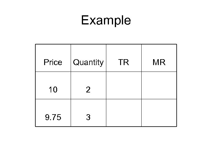
Example Price Quantity 10 2 9. 75 3 TR MR
What differs here from Perfect Competition? ? • Price doesn’t equal MR!!! – Price > MR • Monopolist’s demand curve and marginal revenue curves are DIFFERENT • After the first point Marginal Revenue falls twice as fast as Demand
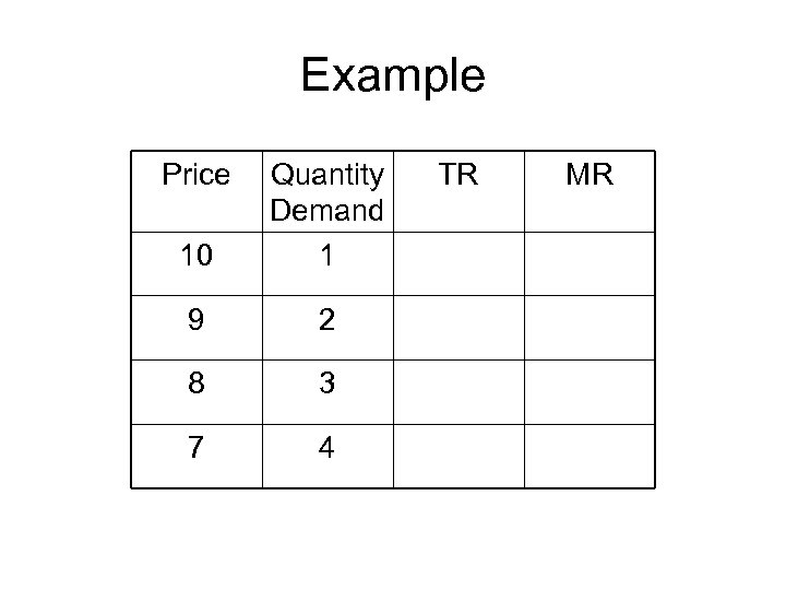
Example Price 10 Quantity Demand 1 9 2 8 3 7 4 TR MR
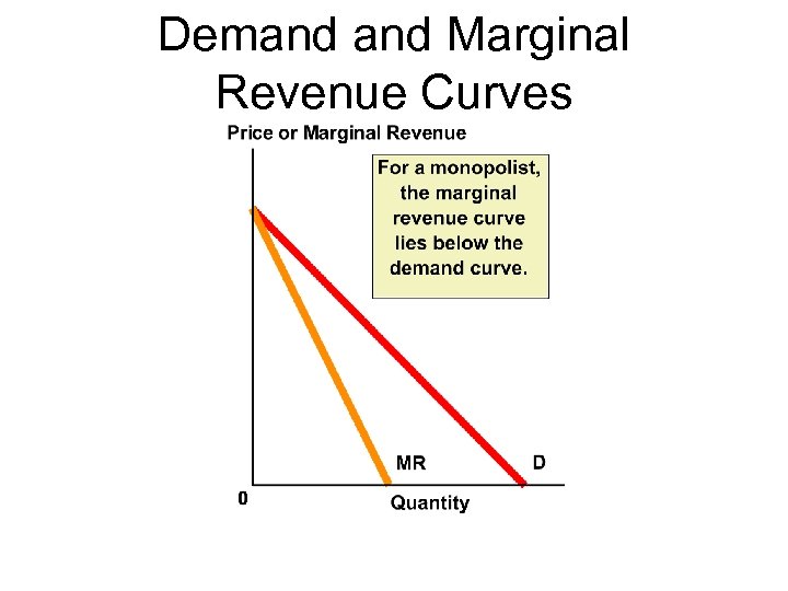
Demand Marginal Revenue Curves
Goal • Profit Maximization • What is the profit maximization rule? – MR = MC • Want to charge the highest price per unit of quantity sold
Monopolist's Profit. Maximizing Price and Quantity of Output
Three cases • P > ATC • P < ATC • P=ATC • Where is AVC? ? – Since monopoly is the industry no need to segment total cost – If suffer a loss can just increase prices to cover the loss
Monopoly Profits and Losses
Differences between monopoly and perfect competition • P = MR for perfect competition but P > MR for monopoly • P = MC for perfect competition but P > MC for monopoly • Monopolist can change prices
Similarities • Both try to maximize profits • Both are constrained by their demand curves • Both equate MR and MC
Long Run Profits • Perfect Competition – Zero Economic Profit (normal profit) • Monopoly – No entry – Profits can be reduced in two ways • Capitalization of profits • Monopoly rent seeking
Capitalization of Profits • Firm owner eventually may sell the business • When sell…include profits into the price – Include in TFC • New owner will face a higher ATC than previous owner – Includes old owner’s profits • Increase in ATC eliminates profit for new owner
Capitalization of Profits
Economic Rent • Profits that can’t be reduced by new entrants • Payment in excess of opportunity cost (profit) • May bring about Rent Seekers – Try to find markets that can gain monopoly status – Time and resources expended to try to get monopoly reduces economic rent
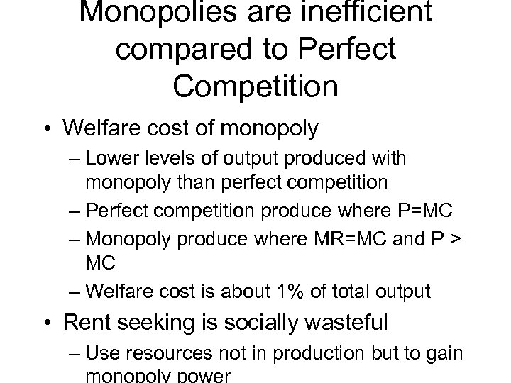
Monopolies are inefficient compared to Perfect Competition • Welfare cost of monopoly – Lower levels of output produced with monopoly than perfect competition – Perfect competition produce where P=MC – Monopoly produce where MR=MC and P > MC – Welfare cost is about 1% of total output • Rent seeking is socially wasteful – Use resources not in production but to gain
Welfare Cost and Rent Seeking as Social Costs of Monopoly
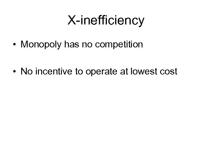
X-inefficiency • Monopoly has no competition • No incentive to operate at lowest cost
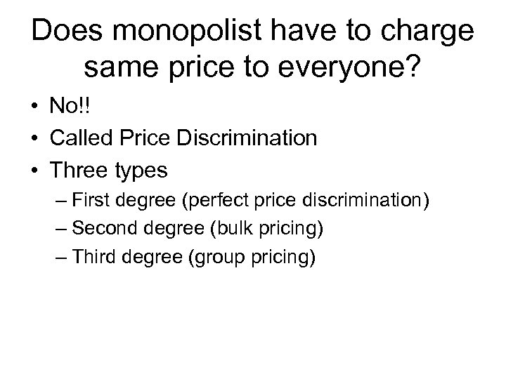
Does monopolist have to charge same price to everyone? • No!! • Called Price Discrimination • Three types – First degree (perfect price discrimination) – Second degree (bulk pricing) – Third degree (group pricing)
Perfect Price discrimination • Highest price willing and able to pay is charged to each person • Price determined by placement on demand curve • Discrimination among units – Ex. Schools
Bulk Pricing • Different prices for different quantities sold • Discrimination among quantities • Ex. costco
Group Pricing • Different prices for different segments of the market • Ex. Senior citizen discounts, coupons, different seats in movie or plane…
Why Price Discriminate? • To gain some of the consumer surplus lost when charge everyone the same price • If successfully perfectly price discriminate – P=MR for all units sold – MR and TR increase – Eliminate consumer surplus
Why doesn’t everyone price discriminate? • Seller must be a price maker • Seller must know each consumer’s willingness to pay • Must be impossible for consumers to resell to others – Arbitrage – Buy for a low price and sell at a higher price
Does a monopolist exhibit resource allocative efficiency? • Perfect competition does!! – P = MC • Monopolist doesn’t!! – P > MC • Perfectly Price Discriminating Monopolist does!! – P = MC
Comparing P. C. Firm, Single-Price Monopolist, & Perfectly Price-Discriminating Monopolist
So does one person paying high prices mean that another can pay low prices? ? • No!! • Perfect Price Discrimination means that each person pays the highest price they are willing and able to pay
Would firms rather be a monopoly? • Yes!! • Rent seekers try to “buy” monopoly positions. • Why? – Fewer constraints on production behavior – Ability to charge different prices to different segments of the population
ea666647937761db04951b2c0dd41073.ppt