782a1574c08c20705d2cdde557c827d0.ppt
- Количество слайдов: 110
 Chapter 7 The Cost of Production
 Topics to be Discussed l Measuring Cost: Which Costs Matter? l Cost in the Short Run l Cost in the Long Run l Long-Run Versus Short-Run Cost Curves © 2005 Pearson Education, Inc. Chapter 7 2
 Topics to be Discussed l Production with Two Outputs: Economies of Scope l Dynamic Changes in Costs: The Learning Curve l Estimating and Predicting Cost © 2005 Pearson Education, Inc. Chapter 7 3
 Introduction l Production technology measures the relationship between input and output l Production technology, together with prices of factor inputs, determine the firm’s cost of production l Given the production technology, managers must choose how to produce © 2005 Pearson Education, Inc. Chapter 7 4
 Introduction l The optimal, cost minimizing, level of inputs can be determined l A firm’s costs depend on the rate of output and we will show these costs are likely to change over time l The characteristics of the firm’s production technology can affect costs in the long run and short run © 2005 Pearson Education, Inc. Chapter 7 5
 Measuring Cost: Which Costs Matter? l For a firm to minimize costs, we must clarify what is meant by costs and how to measure them m It is clear that if a firm has to rent equipment or buildings, the rent they pay is a cost m What if a firm owns its own equipment or building? l How © 2005 Pearson Education, Inc. are costs calculated here? Chapter 7 6
 Measuring Cost: Which Costs Matter? l Accountants tend to take a retrospective view of firms’ costs, whereas economists tend to take a forward-looking view l Accounting Cost m Actual expenses plus depreciation charges for capital equipment l Economic Cost m Cost to a firm of utilizing economic resources in production, including opportunity cost © 2005 Pearson Education, Inc. Chapter 7 7
 Measuring Cost: Which Costs Matter? l Economic costs distinguish between costs the firm can control and those it cannot m Concept of opportunity cost plays an important role l Opportunity cost m Cost associated with opportunities that are foregone when a firm’s resources are not put to their highest-value use © 2005 Pearson Education, Inc. Chapter 7 8
 Opportunity Cost l An Example m. A firm owns its own building and pays no rent for office space m Does this mean the cost of office space is zero? m The building could have been rented instead m Foregone rent is the opportunity cost of using the building for production and should be included in the economic costs of doing business © 2005 Pearson Education, Inc. Chapter 7 9
 Opportunity Cost l A person starting their own business must take into account the opportunity cost of their time m Could have worked elsewhere making a competitive salary l Accountants and economists often treat depreciation differently as well © 2005 Pearson Education, Inc. Chapter 7 10
 Measuring Cost: Which Costs Matter? l Although opportunity costs are hidden and should be taken into account, sunk costs should not l Sunk Cost m Expenditure that has been made and cannot be recovered m Should not influence a firm’s future economic decisions © 2005 Pearson Education, Inc. Chapter 7 11
 Sunk Cost l Firm buys a piece of equipment that cannot be converted to another use l Expenditure on the equipment is a sunk cost m Has no alternative use so cost cannot be recovered – opportunity cost is zero m Decision to buy the equipment might have been good or bad, but now does not matter © 2005 Pearson Education, Inc. Chapter 7 12
 Prospective Sunk Cost l An Example m Firm is considering moving its headquarters m A firm paid $500, 000 for an option to buy a building m The cost of the building is $5 million for a total of $5. 5 million m The firm finds another building for $5. 25 million m Which building should the firm buy? © 2005 Pearson Education, Inc. Chapter 7 13
 Prospective Sunk Cost l Example (cont. ) l The first building should be purchased l The $500, 000 is a sunk cost and should not be considered in the decision to buy l What should be considered is m Spending an additional $5, 250, 000 or m Spending an additional $5, 000 © 2005 Pearson Education, Inc. Chapter 7 14
 Measuring Cost: Which Costs Matter? l Some costs vary with output, while some remain the same no matter the amount of output l Total cost can be divided into: 1. Fixed Cost m Does not vary with the level of output 2. Variable Cost m Cost that varies as output varies © 2005 Pearson Education, Inc. Chapter 7 15
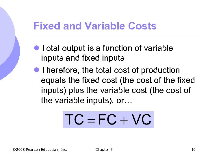 Fixed and Variable Costs l Total output is a function of variable inputs and fixed inputs l Therefore, the total cost of production equals the fixed cost (the cost of the fixed inputs) plus the variable cost (the cost of the variable inputs), or… © 2005 Pearson Education, Inc. Chapter 7 16
 Fixed and Variable Costs l Which costs are variable and which are fixed depends on the time horizon l Short time horizon – most costs are fixed l Long time horizon – many costs become variable l In determining how changes in production will affect costs, must consider if fixed or variable costs are affected. © 2005 Pearson Education, Inc. Chapter 7 17
 Fixed Cost Versus Sunk Cost l Fixed cost and sunk cost are often confused l Fixed Cost m Cost paid by a firm that is in business regardless of the level of output l Sunk Cost m Cost that has been incurred and cannot be recovered © 2005 Pearson Education, Inc. Chapter 7 18
 Measuring Cost: Which Costs Matter? l Personal Computers m Most costs are variable m Largest component: labor l Software m Most costs are sunk m Initial cost of developing the software © 2005 Pearson Education, Inc. Chapter 7 19
 Marginal and Average Cost l In completing a discussion of costs, must also distinguish between m Average Cost m Marginal Cost l After definition of costs is complete, one can consider the analysis between shortrun and long-run costs © 2005 Pearson Education, Inc. Chapter 7 20
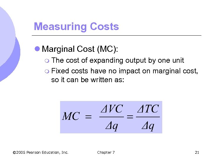 Measuring Costs l Marginal Cost (MC): m The cost of expanding output by one unit m Fixed costs have no impact on marginal cost, so it can be written as: © 2005 Pearson Education, Inc. Chapter 7 21
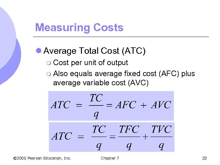 Measuring Costs l Average Total Cost (ATC) m Cost per unit of output m Also equals average fixed cost (AFC) plus average variable cost (AVC) © 2005 Pearson Education, Inc. Chapter 7 22
 Measuring Costs l All the types of costs relevant to production have now been discussed l Can now discuss how they differ in the long and short run l Costs that are fixed in the short run may not be fixed in the long run l Typically in the long run, most if not all costs are variable © 2005 Pearson Education, Inc. Chapter 7 23
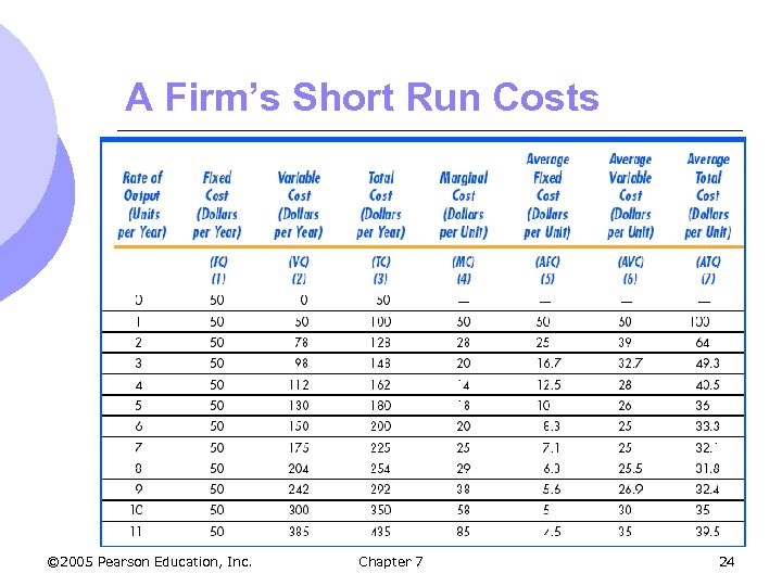 A Firm’s Short Run Costs © 2005 Pearson Education, Inc. Chapter 7 24
 Determinants of Short Run Costs l The rate at which these costs increase depends on the nature of the production process m The extent to which production involves diminishing returns to variable factors l Diminishing returns to labor m When © 2005 Pearson Education, Inc. marginal product of labor is decreasing Chapter 7 25
 Determinants of Short Run Costs l If marginal product of labor decreases significantly as more labor is hired m Costs of production increase rapidly m Greater and greater expenditures must be made to produce more output l If marginal product of labor decreases only slightly as increase labor m Costs will not rise very fast when output is increased © 2005 Pearson Education, Inc. Chapter 7 26
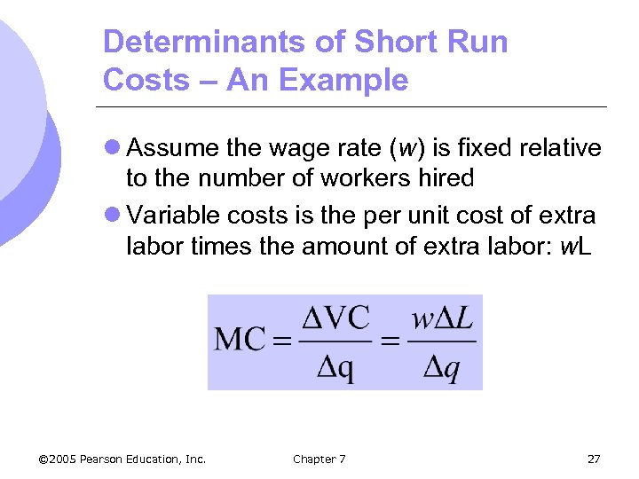 Determinants of Short Run Costs – An Example l Assume the wage rate (w) is fixed relative to the number of workers hired l Variable costs is the per unit cost of extra labor times the amount of extra labor: w. L © 2005 Pearson Education, Inc. Chapter 7 27
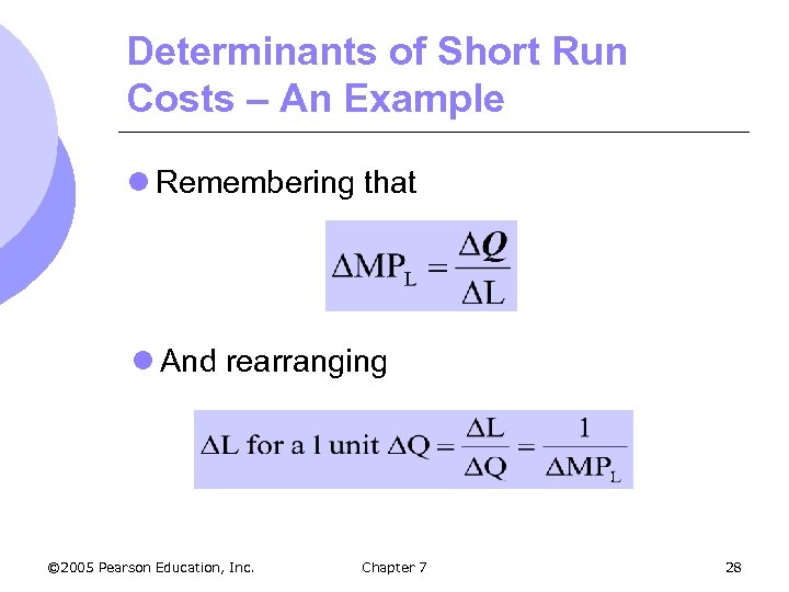 Determinants of Short Run Costs – An Example l Remembering that l And rearranging © 2005 Pearson Education, Inc. Chapter 7 28
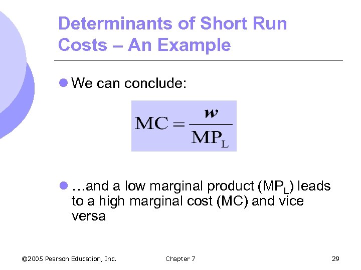 Determinants of Short Run Costs – An Example l We can conclude: l …and a low marginal product (MPL) leads to a high marginal cost (MC) and vice versa © 2005 Pearson Education, Inc. Chapter 7 29
 Determinants of Short Run Costs l Consequently (from the table): m MC l 0 m MC l 5 decreases initially with increasing returns through 4 units of output increases with decreasing returns through 11 units of output © 2005 Pearson Education, Inc. Chapter 7 30
 Cost Curves l The following figures illustrate how various cost measures change as outputs change l Curves based on the information in table 7. 1 discussed earlier © 2005 Pearson Education, Inc. Chapter 7 31
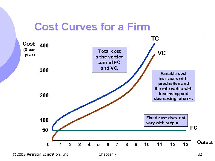 Cost Curves for a Firm TC Cost 400 ($ per year) Total cost is the vertical sum of FC and VC. 300 VC Variable cost increases with production and the rate varies with increasing and decreasing returns. 200 Fixed cost does not vary with output 100 50 0 1 2 © 2005 Pearson Education, Inc. 3 4 5 6 7 Chapter 7 8 9 10 11 12 13 FC Output 32
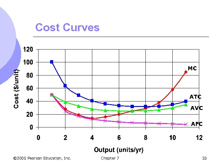 Cost Curves MC ATC AVC AFC © 2005 Pearson Education, Inc. Chapter 7 33
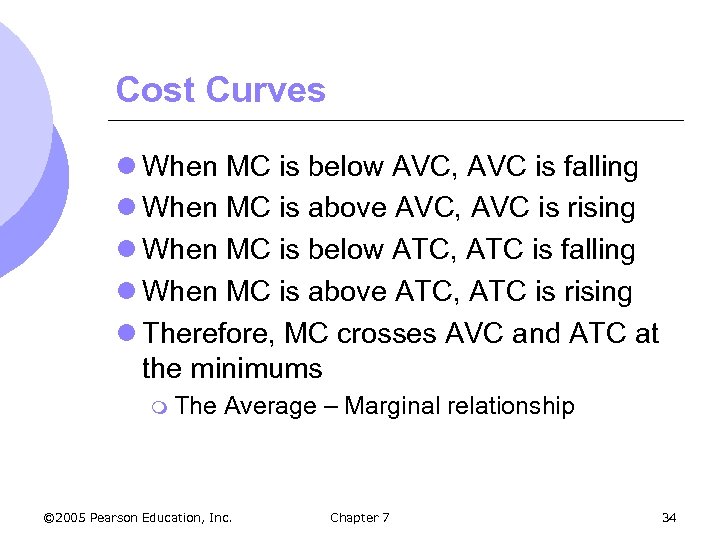 Cost Curves l When MC is below AVC, AVC is falling l When MC is above AVC, AVC is rising l When MC is below ATC, ATC is falling l When MC is above ATC, ATC is rising l Therefore, MC crosses AVC and ATC at the minimums m The Average – Marginal relationship © 2005 Pearson Education, Inc. Chapter 7 34
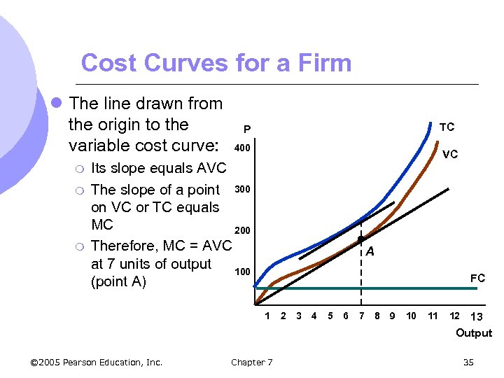 Cost Curves for a Firm l The line drawn from the origin to the variable cost curve: m m m TC P 400 VC Its slope equals AVC The slope of a point 300 on VC or TC equals MC 200 Therefore, MC = AVC at 7 units of output 100 (point A) A FC 1 © 2005 Pearson Education, Inc. Chapter 7 2 3 4 5 6 7 8 9 10 11 12 13 Output 35
 Cost in the Long Run l In the long run a firm can change all of its inputs l In making cost minimizing choices, must look at the cost of using capital and labor in production decisions © 2005 Pearson Education, Inc. Chapter 7 36
 Cost in the Long Run l Capital is either rented/leased or purchased m We will consider capital rented as if it were purchased l Assume Delta is considering purchasing an airplane for $150 million m Plane lasts for 30 years m $5 million per year – economic depreciation for the plane © 2005 Pearson Education, Inc. Chapter 7 37
 Cost in the Long Run l Delta needs to compare its revenues and costs on an annual basis l If the firm had not purchased the plane, it would have earned interest on the $150 million l Forgone interest is an opportunity cost that must be considered © 2005 Pearson Education, Inc. Chapter 7 38
 User Cost of Capital l The user cost of capital must be considered m The annual cost of owning and using the airplane instead of selling or never buying it m Sum of the economic depreciation and the interest (the financial return) that could have been earned had the money been invested elsewhere © 2005 Pearson Education, Inc. Chapter 7 39
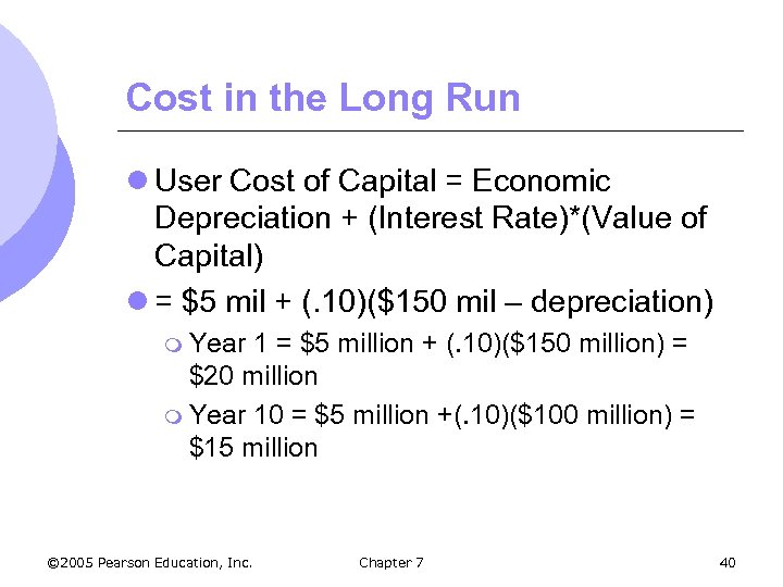 Cost in the Long Run l User Cost of Capital = Economic Depreciation + (Interest Rate)*(Value of Capital) l = $5 mil + (. 10)($150 mil – depreciation) m Year 1 = $5 million + (. 10)($150 million) = $20 million m Year 10 = $5 million +(. 10)($100 million) = $15 million © 2005 Pearson Education, Inc. Chapter 7 40
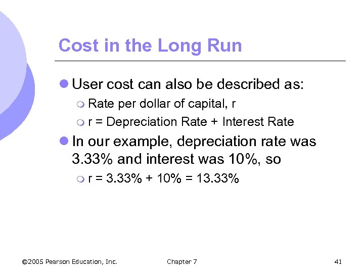 Cost in the Long Run l User cost can also be described as: m Rate per dollar of capital, r m r = Depreciation Rate + Interest Rate l In our example, depreciation rate was 3. 33% and interest was 10%, so mr = 3. 33% + 10% = 13. 33% © 2005 Pearson Education, Inc. Chapter 7 41
 Cost Minimizing Input Choice l How do we put all this together to select inputs to produce a given output at minimum cost? l Assumptions m m m Two Inputs: Labor (L) and capital (K) Price of labor: wage rate (w) The price of capital lr = depreciation rate + interest rate l. Or rental rate if not purchasing l. These are equal in a competitive capital market © 2005 Pearson Education, Inc. Chapter 7 42
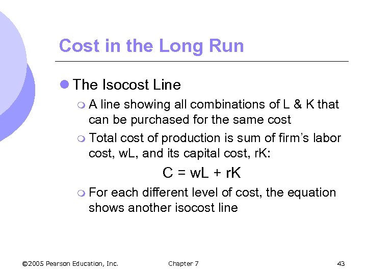 Cost in the Long Run l The Isocost Line m. A line showing all combinations of L & K that can be purchased for the same cost m Total cost of production is sum of firm’s labor cost, w. L, and its capital cost, r. K: C = w. L + r. K m For each different level of cost, the equation shows another isocost line © 2005 Pearson Education, Inc. Chapter 7 43
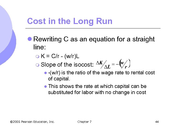 Cost in the Long Run l Rewriting C as an equation for a straight line: m. K = C/r - (w/r)L m Slope of the isocost: l -(w/r) is the ratio of the wage rate to rental cost of capital. l This shows the rate at which capital can be substituted for labor with no change in cost © 2005 Pearson Education, Inc. Chapter 7 44
 Choosing Inputs l We will address how to minimize cost for a given level of output by combining isocosts with isoquants l We choose the output we wish to produce and then determine how to do that at minimum cost m Isoquant is the quantity we wish to produce m Isocost is the combination of K and L that gives a set cost © 2005 Pearson Education, Inc. Chapter 7 45
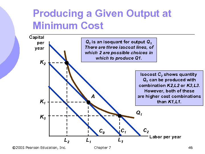 Producing a Given Output at Minimum Cost Capital per year Q 1 is an isoquant for output Q 1. There are three isocost lines, of which 2 are possible choices in which to produce Q 1. K 2 Isocost C 2 shows quantity Q 1 can be produced with combination K 2, L 2 or K 3, L 3. However, both of these are higher cost combinations than K 1, L 1. A K 1 Q 1 K 3 C 0 L 2 © 2005 Pearson Education, Inc. C 1 L 3 L 1 Chapter 7 C 2 Labor per year 46
 Input Substitution When an Input Price Change l If the price of labor changes, then the slope of the isocost line changes, -(w/r) l It now takes a new quantity of labor and capital to produce the output l If price of labor increases relative to price of capital, and capital is substituted for labor © 2005 Pearson Education, Inc. Chapter 7 47
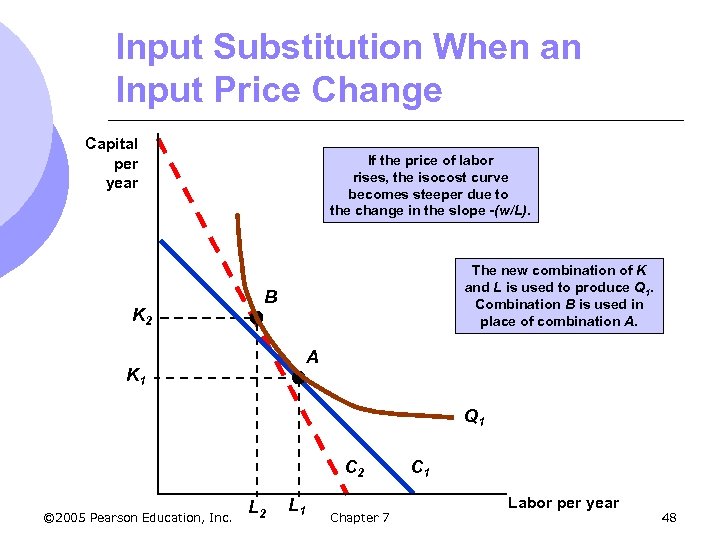 Input Substitution When an Input Price Change Capital per year K 2 If the price of labor rises, the isocost curve becomes steeper due to the change in the slope -(w/L). The new combination of K and L is used to produce Q 1. Combination B is used in place of combination A. B A K 1 Q 1 C 2 © 2005 Pearson Education, Inc. L 2 L 1 Chapter 7 C 1 Labor per year 48
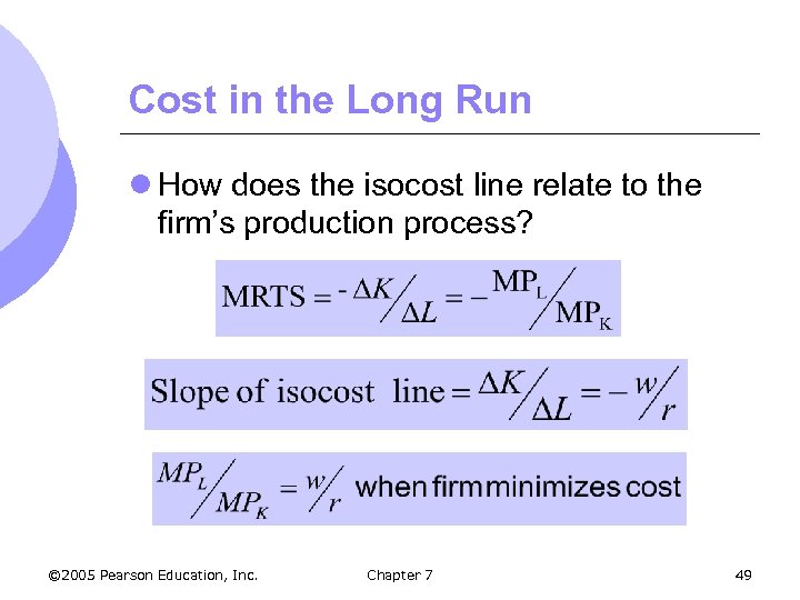 Cost in the Long Run l How does the isocost line relate to the firm’s production process? © 2005 Pearson Education, Inc. Chapter 7 49
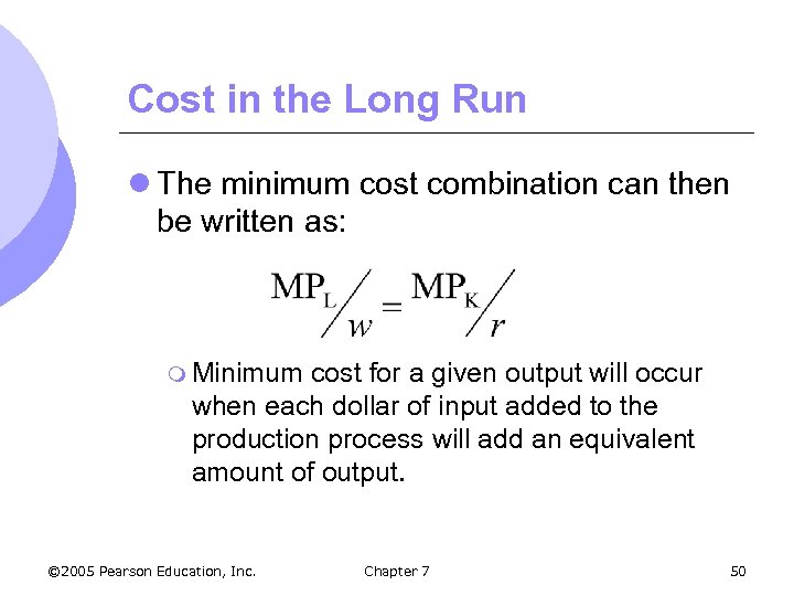 Cost in the Long Run l The minimum cost combination can then be written as: m Minimum cost for a given output will occur when each dollar of input added to the production process will add an equivalent amount of output. © 2005 Pearson Education, Inc. Chapter 7 50
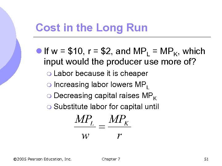 Cost in the Long Run l If w = $10, r = $2, and MPL = MPK, which input would the producer use more of? m Labor because it is cheaper m Increasing labor lowers MPL m Decreasing capital raises MPK m Substitute labor for capital until © 2005 Pearson Education, Inc. Chapter 7 51
 Cost in the Long Run l Cost minimization with Varying Output Levels m For each level of output, there is an isocost curve showing minimum cost for that output level m A firm’s expansion path shows the minimum cost combinations of labor and capital at each level of output m Slope equals K/ L © 2005 Pearson Education, Inc. Chapter 7 52
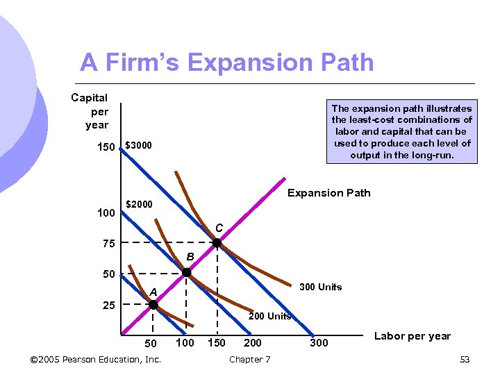 A Firm’s Expansion Path Capital per year The expansion path illustrates the least-cost combinations of labor and capital that can be used to produce each level of output in the long-run. 150 $3000 Expansion Path 100 $2000 C 75 B 50 300 Units A 25 200 Units 50 © 2005 Pearson Education, Inc. 100 150 200 Chapter 7 300 Labor per year 53
 Expansion Path and Long Run Costs l Firm’s expansion path has same information as long-run total cost curve l To move from expansion path to LR cost curve m Find tangency with isoquant and isocost m Determine min cost of producing the output level selected m Graph output-cost combination © 2005 Pearson Education, Inc. Chapter 7 54
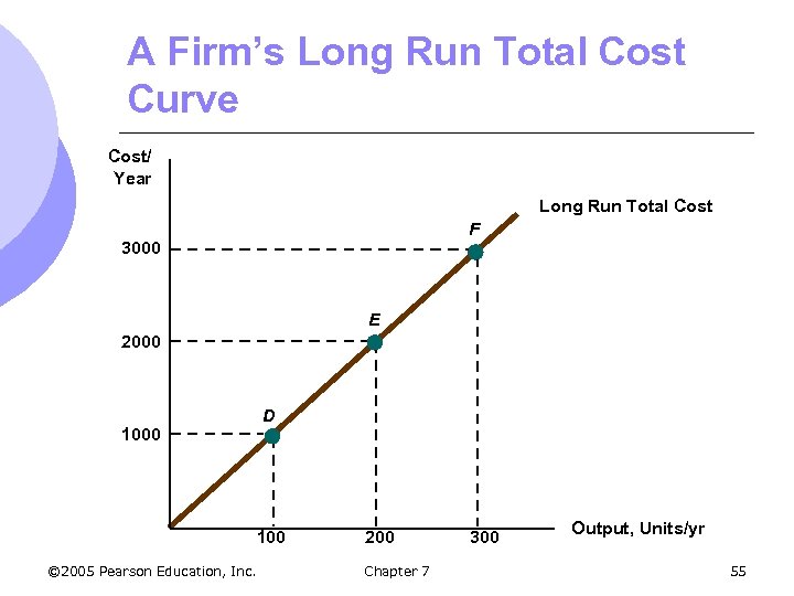 A Firm’s Long Run Total Cost Curve Cost/ Year Long Run Total Cost F 3000 E 2000 D 1000 100 © 2005 Pearson Education, Inc. 200 Chapter 7 300 Output, Units/yr 55
 Long Run Versus Short Run Cost Curves l In the short run, some costs are fixed l In the long run, firm can change anything including plant size m Can produce at a lower average cost in long run than in short run m Capital and labor are both flexible l We can show this by holding capital fixed in the short run and flexible in long run © 2005 Pearson Education, Inc. Chapter 7 56
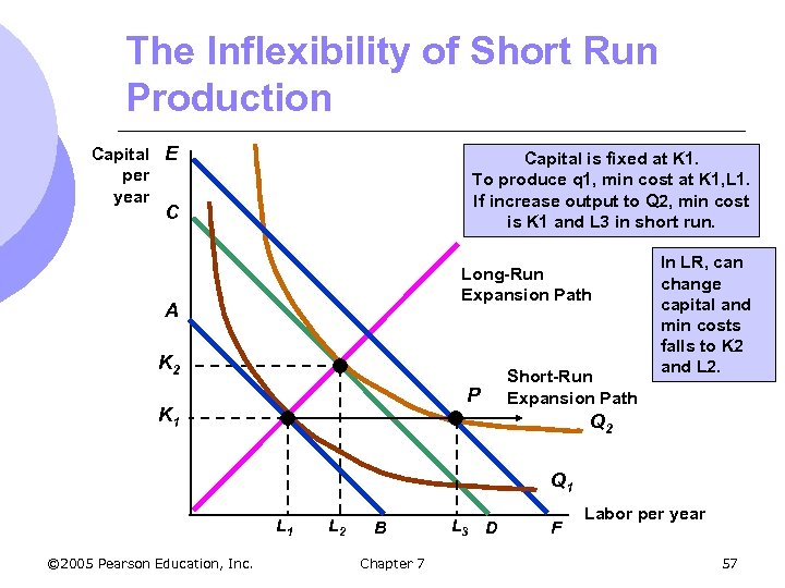 The Inflexibility of Short Run Production Capital E per year Capital is fixed at K 1. To produce q 1, min cost at K 1, L 1. If increase output to Q 2, min cost is K 1 and L 3 in short run. C Long-Run Expansion Path A K 2 P K 1 Short-Run Expansion Path In LR, can change capital and min costs falls to K 2 and L 2. Q 2 Q 1 L 1 © 2005 Pearson Education, Inc. L 2 B Chapter 7 L 3 D F Labor per year 57
 Long Run Versus Short Run Cost Curves l Long-Run Average Cost (LAC) m Most important determinant of the shape of the LR AC and MC curves is relationship between scale of the firm’s operation and inputs required to minimize cost 1. Constant Returns to Scale m m If input is doubled, output will double AC cost is constant at all levels of output © 2005 Pearson Education, Inc. Chapter 7 58
 Long Run Versus Short Run Cost Curves 2. Increasing Returns to Scale m m If input is doubled, output will more than double AC decreases at all levels of output 3. Decreasing Returns to Scale m m If input is doubled, output will less than double AC increases at all levels of output © 2005 Pearson Education, Inc. Chapter 7 59
 Long Run Versus Short Run Cost Curves l In the long run: m Firms experience increasing and decreasing returns to scale and therefore long-run average cost is “U” shaped. m Source of U-shape is due to returns to scale instead of decreasing returns to scale like the short-run curve m Long-run marginal cost curve measures the change in long-run total costs as output is increased by 1 unit © 2005 Pearson Education, Inc. Chapter 7 60
 Long Run Versus Short Run Cost Curves l Long-run marginal cost leads long-run average cost: m If LMC < LAC, LAC will fall m If LMC > LAC, LAC will rise m Therefore, LMC = LAC at the minimum of LAC l In special case where LAC is constant, LAC and LMC are equal © 2005 Pearson Education, Inc. Chapter 7 61
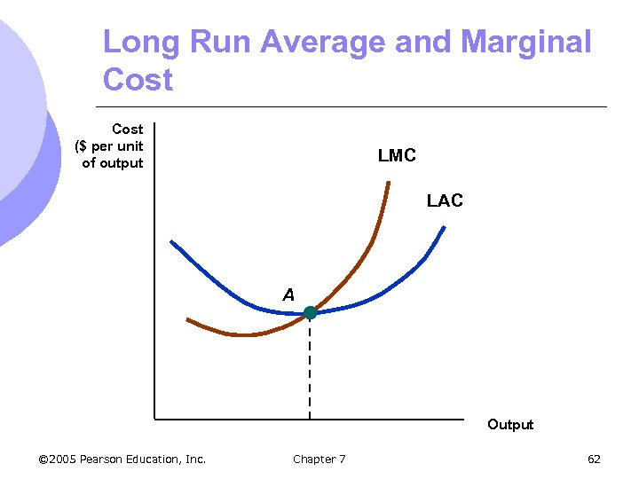 Long Run Average and Marginal Cost ($ per unit of output LMC LAC A Output © 2005 Pearson Education, Inc. Chapter 7 62
 Long Run Costs l As output increases, firm’s AC of producing is likely to decline to a point 1. 2. 3. On a larger scale, workers can better specialize Scale can provide flexibility – managers can organize production more effectively Firm may be able to get inputs at lower cost if can get quantity discounts. Lower prices might lead to different input mix. © 2005 Pearson Education, Inc. Chapter 7 63
 Long Run Costs l At some point, AC will begin to increase 1. 2. 3. Factory space and machinery make it more difficult for workers to do their jobs efficiently Managing a larger firm may become more complex and inefficient as the number of tasks increase Bulk discounts can no longer be utilized. Limited availability of inputs may cause price to rise. © 2005 Pearson Education, Inc. Chapter 7 64
 Long Run Costs l When input proportions change, the firm’s expansion path is no longer a straight line m Concept of return to scale no longer applies l Economies of scale reflects input proportions that change as the firm changes its level of production © 2005 Pearson Education, Inc. Chapter 7 65
 Economies and Diseconomies of Scale l Economies of Scale m Increase in output is greater than the increase in inputs l Diseconomies of Scale m Increase inputs in output is less than the increase in l U-shaped LAC shows economies of scale for relatively low output levels and diseconomies of scale for higher levels © 2005 Pearson Education, Inc. Chapter 7 66
 Long Run Costs l Increasing Returns to Scale m Output more than doubles when the quantities of all inputs are doubled l Economies of Scale m Doubling of output requires less than a doubling of cost © 2005 Pearson Education, Inc. Chapter 7 67
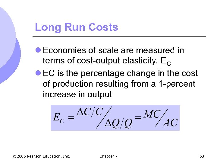 Long Run Costs l Economies of scale are measured in terms of cost-output elasticity, EC l EC is the percentage change in the cost of production resulting from a 1 -percent increase in output © 2005 Pearson Education, Inc. Chapter 7 68
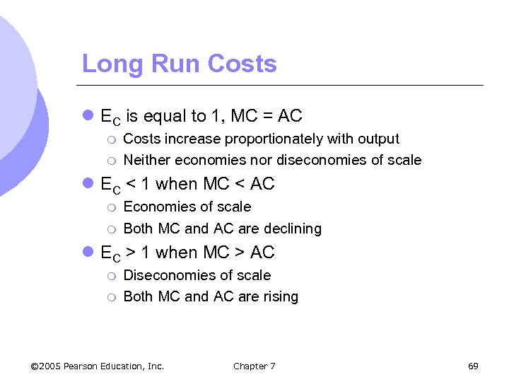 Long Run Costs l EC is equal to 1, MC = AC m m Costs increase proportionately with output Neither economies nor diseconomies of scale l EC < 1 when MC < AC m m Economies of scale Both MC and AC are declining l EC > 1 when MC > AC m m Diseconomies of scale Both MC and AC are rising © 2005 Pearson Education, Inc. Chapter 7 69
 Long Run Versus Short Run Cost Curves l We will use short and long run costs to determine the optimal plant size l We can show the short run average costs for 3 different plant sizes l This decision is important because once built, the firm may not be able to change plant size for a while © 2005 Pearson Education, Inc. Chapter 7 70
 Long Run Cost with Constant Returns to Scale l The optimal plant size will depend on the anticipated output m If expect to produce q 0, then should build smallest plant: AC = $8 m If produce more, like q 1, AC rises m If expect to produce q 2, middle plant is least cost m If expect to produce q 3, largest plant is best © 2005 Pearson Education, Inc. Chapter 7 71
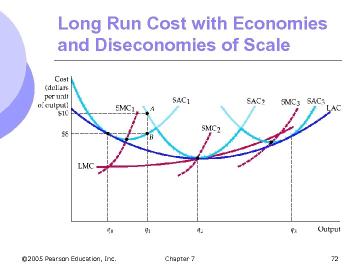 Long Run Cost with Economies and Diseconomies of Scale © 2005 Pearson Education, Inc. Chapter 7 72
 Long Run Cost with Constant Returns to Scale l What is the firm’s long run cost curve? m Firms can change scale to change output in the long run m The long run cost curve is the dark blue portion of the SAC curve which represents the minimum cost for any level of output m Firm will always choose plant that minimizes the average cost of production © 2005 Pearson Education, Inc. Chapter 7 73
 Long Run Cost with Constant Returns to Scale l The long-run average cost curve envelops the short-run average cost curves l The LAC curve exhibits economies of scale initially but exhibits diseconomies at higher output levels © 2005 Pearson Education, Inc. Chapter 7 74
 Production with Two Outputs – Economies of Scope l Many firms produce more than one product and those products are closely linked l Examples: m Chicken farm--poultry and eggs m Automobile company--cars and trucks m University--teaching and research © 2005 Pearson Education, Inc. Chapter 7 75
 Production with Two Outputs – Economies of Scope l Advantages 1. Both use capital and labor 2. The firms share management resources 3. Both use the same labor skills and types of machinery © 2005 Pearson Education, Inc. Chapter 7 76
 Production with Two Outputs – Economies of Scope l Firms must choose how much of each to produce l The alternative quantities can be illustrated using product transformation curves m Curves showing the various combinations of two different outputs (products) that can be produced with a given set of inputs © 2005 Pearson Education, Inc. Chapter 7 77
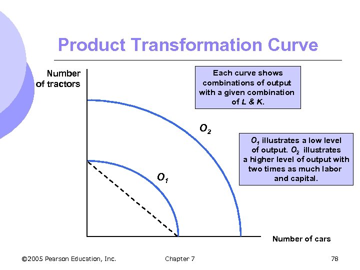 Product Transformation Curve Number of tractors Each curve shows combinations of output with a given combination of L & K. O 2 O 1 illustrates a low level of output. O 2 illustrates a higher level of output with two times as much labor and capital. Number of cars © 2005 Pearson Education, Inc. Chapter 7 78
 Product Transformation Curve l Product transformation curves are negatively sloped m To get more of one output, must give up some of the other output l Constant returns exist in this example m Second curve lies twice as far from origin as the first curve l Curve is concave m Joint © 2005 Pearson Education, Inc. production has its advantages Chapter 7 79
 Production with Two Outputs – Economies of Scope l There is no direct relationship between economies of scope and economies of scale m May experience economies of scope and diseconomies of scale m May have economies of scale and not have economies of scope © 2005 Pearson Education, Inc. Chapter 7 80
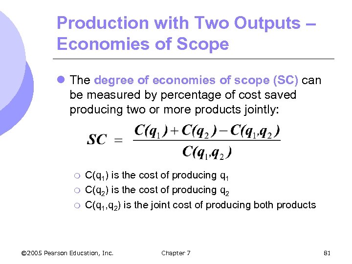 Production with Two Outputs – Economies of Scope l The degree of economies of scope (SC) can be measured by percentage of cost saved producing two or more products jointly: m m m C(q 1) is the cost of producing q 1 C(q 2) is the cost of producing q 2 C(q 1, q 2) is the joint cost of producing both products © 2005 Pearson Education, Inc. Chapter 7 81
 Production with Two Outputs – Economies of Scope l With economies of scope, the joint cost is less than the sum of the individual costs l Interpretation: m If SC > 0 Economies of scope m If SC < 0 Diseconomies of scope m The greater the value of SC, the greater the economies of scope © 2005 Pearson Education, Inc. Chapter 7 82
 Dynamic Changes in Costs – The Learning Curve l Firms may lower their costs not only due to economies of scope, but also due to managers and workers becoming more experienced at their jobs l As management and labor gain experience with production, the firm’s marginal and average costs may fall © 2005 Pearson Education, Inc. Chapter 7 83
 Dynamic Changes in Costs – The Learning Curve l Reasons 1. 2. 3. 4. Speed of work increases with experience Managers learn to schedule production processes more efficiently More flexibility is allowed with experience; may include more specialized tools and plant organization Suppliers become more efficient, passing savings to company © 2005 Pearson Education, Inc. Chapter 7 84
 Dynamic Changes in Costs – The Learning Curve l The learning curve measures the impact of workers’ experience on the costs of production l It describes the relationship between a firm’s cumulative output and the amount of inputs needed to produce a unit of output © 2005 Pearson Education, Inc. Chapter 7 85
 The Learning Curve Hours of labor per machine lot 10 8 6 4 2 0 10 © 2005 Pearson Education, Inc. 20 30 Chapter 7 40 50 Cumulative number of machine lots produced 86
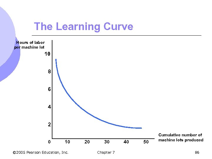
 The Learning Curve l The horizontal axis measures the cumulative number of hours of machine tools the firm has produced l The vertical axis measures the number of hours of labor needed to produce each lot © 2005 Pearson Education, Inc. Chapter 7 87
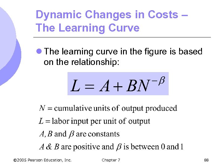 Dynamic Changes in Costs – The Learning Curve l The learning curve in the figure is based on the relationship: © 2005 Pearson Education, Inc. Chapter 7 88
 Dynamic Changes in Costs – The Learning Curve l If N = 1 m. L equals A + B and this measures labor input to produce the first unit of output l If = 0 m Labor input per unit of output remains constant as the cumulative level of output increases, so there is no learning © 2005 Pearson Education, Inc. Chapter 7 89
 Dynamic Changes in Costs – The Learning Curve l If > 0 and N increases, m. L approaches A, and A represents minimum labor input/unit of output after all learning has taken place l The larger , m The more important the learning effect © 2005 Pearson Education, Inc. Chapter 7 90
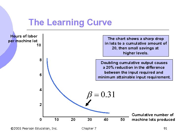 The Learning Curve Hours of labor per machine lot 10 The chart shows a sharp drop in lots to a cumulative amount of 20, then small savings at higher levels. 8 Doubling cumulative output causes a 20% reduction in the difference between the input required and minimum attainable input requirement. 6 4 2 0 10 © 2005 Pearson Education, Inc. 20 30 Chapter 7 40 50 Cumulative number of machine lots produced 91
 Dynamic Changes in Costs – The Learning Curve l Observations 1. New firms may experience a learning curve, not economies of scale l 2. Should increase production of many lots regardless of individual lot size Older firms have relatively small gains from learning l Should produce their machines in very large lots to take advantage of lower costs associated with size © 2005 Pearson Education, Inc. Chapter 7 92
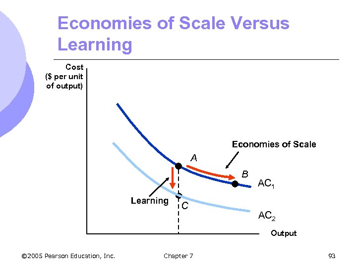 Economies of Scale Versus Learning Cost ($ per unit of output) Economies of Scale A B Learning C AC 1 AC 2 Output © 2005 Pearson Education, Inc. Chapter 7 93
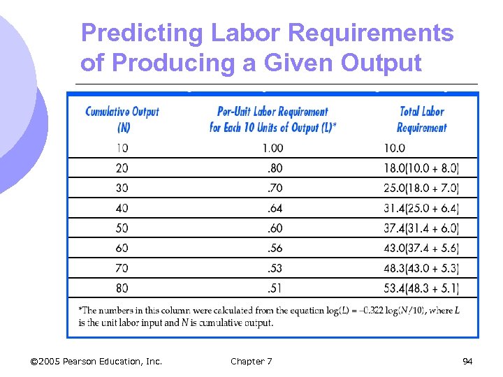 Predicting Labor Requirements of Producing a Given Output © 2005 Pearson Education, Inc. Chapter 7 94
 Dynamic Changes in Costs – The Learning Curve l From the table, the learning curve implies: 1. 2. 3. The labor requirement falls per unit Costs will be high at first and then will fall with learning After 8 years, the labor requirement will be 0. 51 and per unit cost will be half what it was in the first year of production © 2005 Pearson Education, Inc. Chapter 7 95
 The Learning Curve in Practice l Scenario m A new firm enters the chemical processing industry l Do they: 1. 2. Produce a low level of output and sell at a high price? Produce a high level of output and sell at a low price? © 2005 Pearson Education, Inc. Chapter 7 96
 The Learning Curve in Practice l The Empirical Findings m Study of 37 chemical products l Average cost fell 5. 5% per year l For each doubling of plant size, average production costs fall by 11% l For each doubling of cumulative output, the average cost of production falls by 27% l Which is more important, the economies of scale or learning effects? © 2005 Pearson Education, Inc. Chapter 7 97
 The Learning Curve in Practice l Other Empirical Findings m In the semiconductor industry, a study of seven generations of DRAM semiconductors from 1974 -1992 found learning rates averaged 20% m In the aircraft industry, the learning rates are as high as 40% © 2005 Pearson Education, Inc. Chapter 7 98
 The Learning Curve in Practice l Applying Learning Curves 1. 2. To determine if it is profitable to enter an industry To determine when profits will occur based on plant size and cumulative output © 2005 Pearson Education, Inc. Chapter 7 99
 Estimating and Predicting Cost l Estimates of future costs can be obtained from a cost function, which relates the cost of production to the level of output and other variables that the firm can control l Suppose we wanted to derive the total cost curve for automobile production © 2005 Pearson Education, Inc. Chapter 7 100
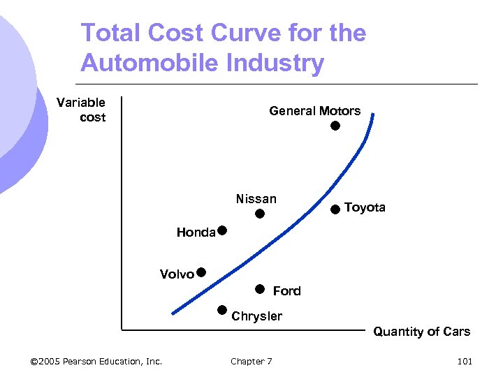 Total Cost Curve for the Automobile Industry Variable cost General Motors Nissan Toyota Honda Volvo Ford Chrysler Quantity of Cars © 2005 Pearson Education, Inc. Chapter 7 101
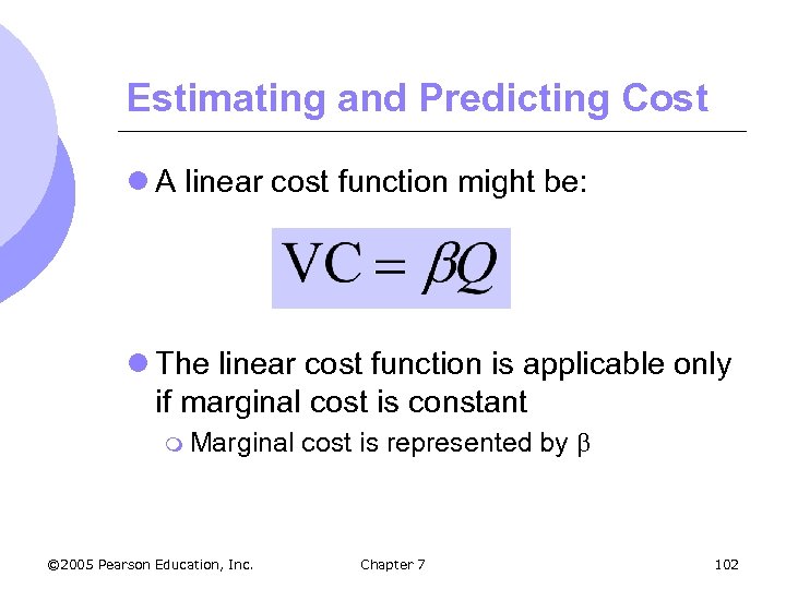 Estimating and Predicting Cost l A linear cost function might be: l The linear cost function is applicable only if marginal cost is constant m Marginal © 2005 Pearson Education, Inc. cost is represented by Chapter 7 102
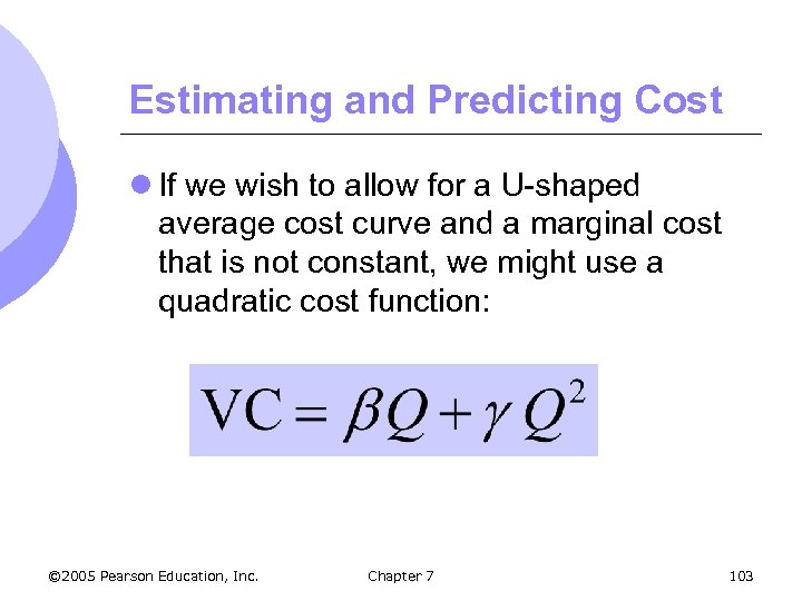 Estimating and Predicting Cost l If we wish to allow for a U-shaped average cost curve and a marginal cost that is not constant, we might use a quadratic cost function: © 2005 Pearson Education, Inc. Chapter 7 103
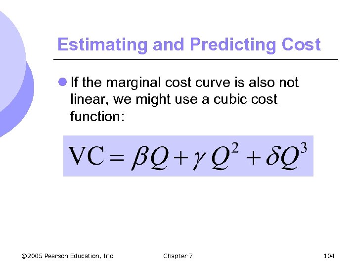 Estimating and Predicting Cost l If the marginal cost curve is also not linear, we might use a cubic cost function: © 2005 Pearson Education, Inc. Chapter 7 104
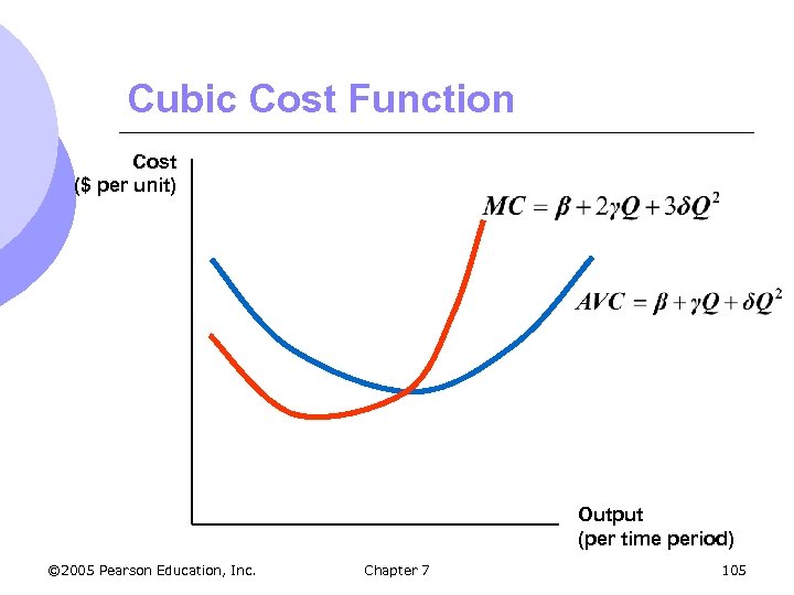 Cubic Cost Function Cost ($ per unit) Output (per time period) © 2005 Pearson Education, Inc. Chapter 7 105
 Estimating and Predicting Cost l Difficulties in Measuring Cost 1. 2. 3. Output data may represent an aggregate of different types of products Cost data may not include opportunity cost Allocating cost to a particular product may be difficult when there is more than one product line © 2005 Pearson Education, Inc. Chapter 7 106
 Cost Functions & Measurement of Scale Economies l Scale Economy Index (SCI) m EC = 1, SCI = 0: no economies or diseconomies of scale m EC > 1, SCI is negative: diseconomies of scale m EC < 1, SCI is positive: economies of scale © 2005 Pearson Education, Inc. Chapter 7 107
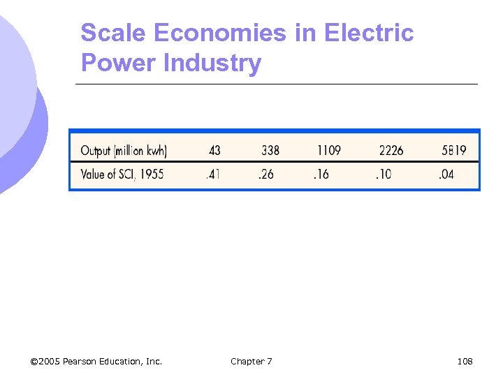 Scale Economies in Electric Power Industry © 2005 Pearson Education, Inc. Chapter 7 108
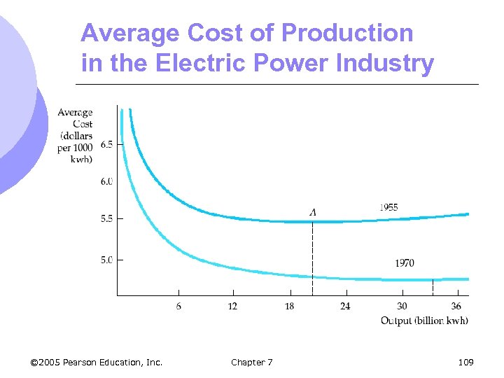 Average Cost of Production in the Electric Power Industry © 2005 Pearson Education, Inc. Chapter 7 109
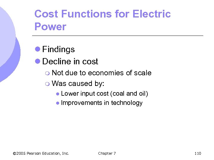 Cost Functions for Electric Power l Findings l Decline in cost m Not due to economies of scale m Was caused by: l Lower input cost (coal and oil) l Improvements in technology © 2005 Pearson Education, Inc. Chapter 7 110


