45b0e33d16e0122b2253d2b35a8bb811.ppt
- Количество слайдов: 92
Chapter 7 Random Variables and Discrete probability Distributions 7 -1
Random Variables A random variable(隨機變數) is a function or rule that assigns a number to each outcome of an experiment. n Alternatively, the value of a random variable is a numerical event. n A random variable reflects the aspect of a random experiment that is of interest for us. n Instead of talking about the coin flipping event as {heads, tails} think of it as “the number of heads when flipping a coin” {1, 0} (numerical events) n 2007會計資訊系統計學 (一)上課投影片 2
Variables n n n There are two types of random variables: n Discrete random variable n Continuous random variable. Discrete Random Variable(間斷 、離散型隨機變數) – one that takes on a countable number of values – E. g. values on the roll of dice: 2, 3, 4, …, 12 Continuous Random Variable (連續型隨機變數) – one whose values are not discrete, not countable – E. g. time (30. 1 minutes? 30. 10000001 minutes? ) Analogy: Integers are Discrete, while Real Numbers are Continuous n 2007會計資訊系統計學 (一)上課投影片 3
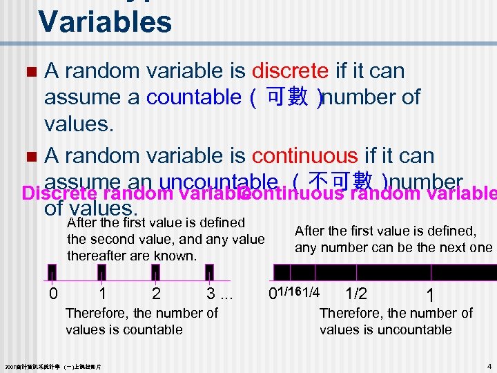
Variables A random variable is discrete if it can assume a countable(可數) number of values. n A random variable is continuous if it can assume an uncountable (不可數) variable number Discrete random variable Continuous random of values. n After the first value is defined the second value, and any value thereafter are known. 0 1 2 3. . . Therefore, the number of values is countable 2007會計資訊系統計學 (一)上課投影片 After the first value is defined, any number can be the next one 01/161/4 1/2 1 Therefore, the number of values is uncountable 4
Probability Distributions n n A probability distribution(機率分配) is a table, formula, or graph that describes the values of a random variable and the probability associated with these values. Since we’re describing a random variable (which can be discrete or continuous) we have two types of probability distributions: – Discrete Probability Distribution, (this chapter) and – Continuous Probability Distribution 2007會計資訊系統計學 (一)上課投影片 5
Probability Notation n An upper-case letter will represent the name of the random variable, usually X. n Its lower-case counterpart will represent the value of the random variable. The probability that the random variable X will equal x is: P(X = x) n or more simply P(x) n 2007會計資訊系統計學 (一)上課投影片 6
Distributions n A table, formula, or graph that lists all possible values a discrete random variable can assume, together with associated probabilities, is called a discrete probability distribution. n To calculate the probability that the random variable X assumes the value x, P(X = x), add the probabilities of all the simple events for which X is equal to x, or n use probability calculation tools (tree diagram), n apply probability definitions n 2007會計資訊系統計學 (一)上課投影片 7
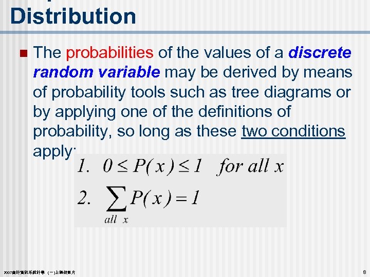
Distribution n The probabilities of the values of a discrete random variable may be derived by means of probability tools such as tree diagrams or by applying one of the definitions of probability, so long as these two conditions apply: 2007會計資訊系統計學 (一)上課投影片 8
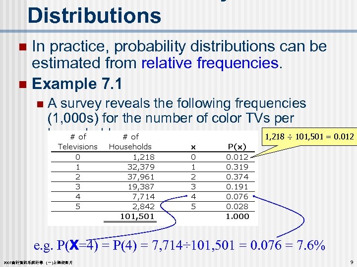
Distributions In practice, probability distributions can be estimated from relative frequencies. n Example 7. 1 n n A survey reveals the following frequencies (1, 000 s) for the number of color TVs per household. 1, 218 ÷ 101, 501 = 0. 012 e. g. P(X=4) = P(4) = 7, 714÷ 101, 501 = 0. 076 = 7. 6% 2007會計資訊系統計學 (一)上課投影片 9
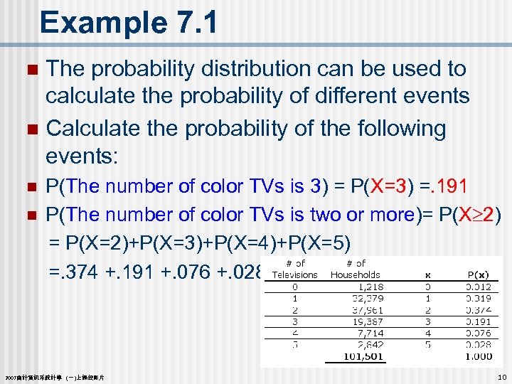
Example 7. 1 The probability distribution can be used to calculate the probability of different events n Calculate the probability of the following events: n P(The number of color TVs is 3) = P(X=3) =. 191 n P(The number of color TVs is two or more)= P(X³ 2) = P(X=2)+P(X=3)+P(X=4)+P(X=5) =. 374 +. 191 +. 076 +. 028 =. 669 n 2007會計資訊系統計學 (一)上課投影片 10
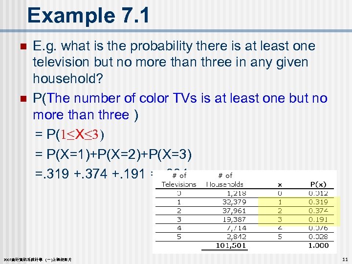
Example 7. 1 E. g. what is the probability there is at least one television but no more than three in any given household? n P(The number of color TVs is at least one but no more than three ) = P(1≤X≤ 3) = P(X=1)+P(X=2)+P(X=3) =. 319 +. 374 +. 191 =. 884 n 2007會計資訊系統計學 (一)上課投影片 11
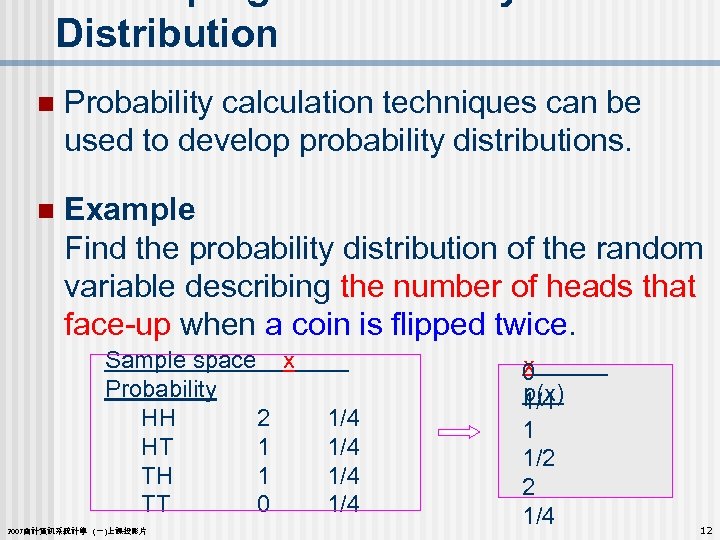
Distribution n Probability calculation techniques can be used to develop probability distributions. n Example Find the probability distribution of the random variable describing the number of heads that face-up when a coin is flipped twice. Sample space x Probability HH 2 1/4 HT 1 1/4 TH 1 1/4 TT 0 1/4 2007會計資訊系統計學 (一)上課投影片 x 0 p(x) 1/4 1 1/2 2 1/4 12
Example 7. 2 A mutual fund sales person knows that there is 20% chance of closing a sale on each call she makes. n What is the probability distribution of the number of sales if she plans to call three customers? n Let S denote success, i. e. closing a sale P(S)=. 20 n Thus SC is not closing a sale, and P(SC)=. 80 n Let X denote the number of sales , X=0, 1, 2, 3. n 2007會計資訊系統計學 (一)上課投影片 13
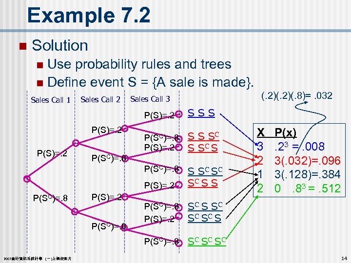
Example 7. 2 n Solution Use probability rules and trees n Define event S = {A sale is made}. n Sales Call 1 Sales Call 2 (. 2)(. 8)=. 032 Sales Call 3 P(S)=. 2 P(SC)=. 8 P(S)=. 2 SC S S C SC SC SC P(SC)=. 8 P(S)=. 2 P(SC)=. 8 2007會計資訊系統計學 (一)上課投影片 S S C SC SC S S P(SC)=. 8 S S SC S P(S)=. 2 P(SC)=. 8 P(S)=. 2 SSS X 3 2 1 2 P(x). 23 =. 008 3(. 032)=. 096 3(. 128)=. 384 0. 83 =. 512 14
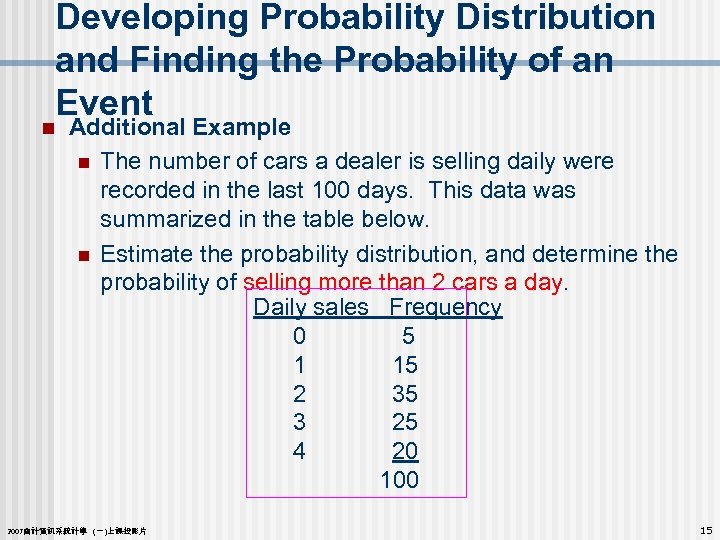
Developing Probability Distribution and Finding the Probability of an Event n Additional Example n The number of cars a dealer is selling daily were recorded in the last 100 days. This data was summarized in the table below. n Estimate the probability distribution, and determine the probability of selling more than 2 cars a day. Daily sales Frequency 0 5 1 15 2 35 3 25 4 20 100 2007會計資訊系統計學 (一)上課投影片 15
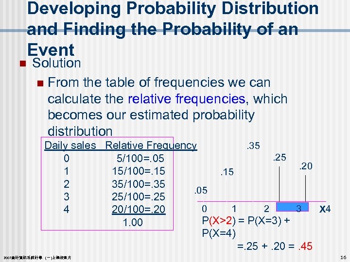
Developing Probability Distribution and Finding the Probability of an Event n Solution n From the table of frequencies we can calculate the relative frequencies, which becomes our estimated probability distribution . 35 Daily sales Relative Frequency. 25 0 5/100=. 05. 20 1 15/100=. 15 2 35/100=. 35. 05 3 25/100=. 25 0 1 2 3 4 X 4 20/100=. 20 P(X>2) = P(X=3) + 1. 00 P(X=4) =. 25 +. 20 =. 45 2007會計資訊系統計學 (一)上課投影片 16
Distribution n The discrete probability distribution represents a population(母體) • • Example 7. 1 the population of number of TVs per household Example 7. 2 the population of sales call outcomes n Since we have populations, we can describe them by computing various parameters(參數). n E. g. the population mean and population 2007會計資訊系統計學 (一)上課投影片 17
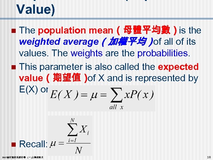
Value) The population mean(母體平均數) is the weighted average(加權平均) of all of its values. The weights are the probabilities. n This parameter is also called the expected value(期望值) of X and is represented by E(X) or µ. n n Recall: 2007會計資訊系統計學 (一)上課投影片 18
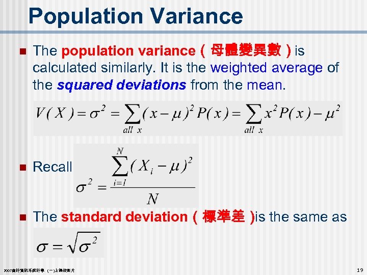
Population Variance n The population variance(母體變異數) is calculated similarly. It is the weighted average of the squared deviations from the mean. n Recall: n The standard deviation(標準差) is the same as before: 2007會計資訊系統計學 (一)上課投影片 19
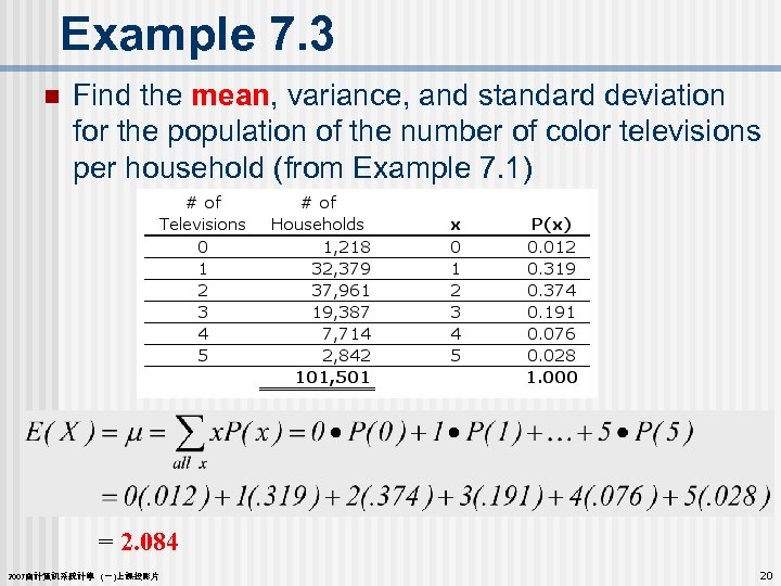
Example 7. 3 n Find the mean, variance, and standard deviation for the population of the number of color televisions per household (from Example 7. 1) = 2. 084 2007會計資訊系統計學 (一)上課投影片 20
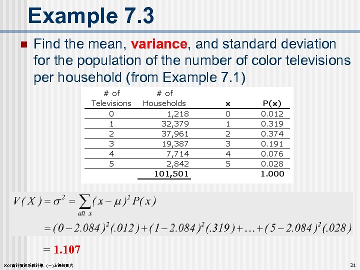
Example 7. 3 n Find the mean, variance, and standard deviation for the population of the number of color televisions per household (from Example 7. 1) = 1. 107 2007會計資訊系統計學 (一)上課投影片 21
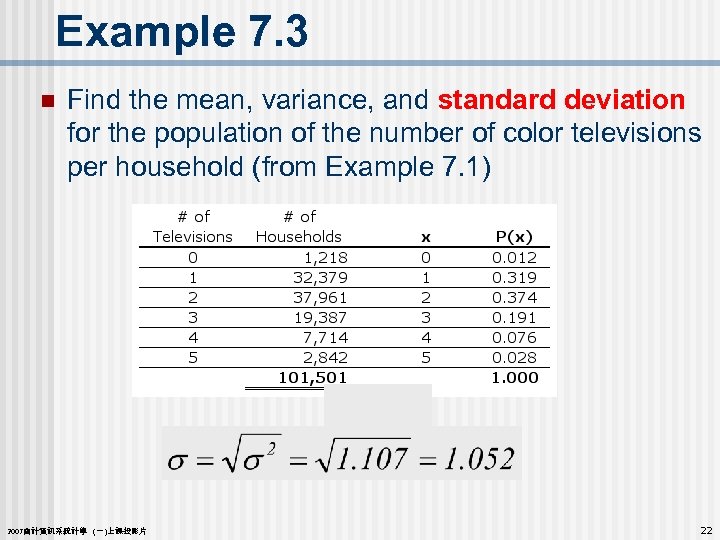
Example 7. 3 n Find the mean, variance, and standard deviation for the population of the number of color televisions per household (from Example 7. 1) 2007會計資訊系統計學 (一)上課投影片 22
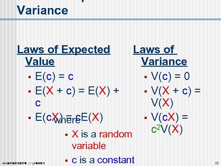
Variance Laws of Expected Laws of Value Variance § E(c) = c § V(c) = 0 § E(X + c) = E(X) + § V(X + c) = c V(X) § E(c. X) = c. E(X) § V(c. X) = where c 2 V(X) § X is a random 2007會計資訊系統計學 (一)上課投影片 § variable c is a constant 23
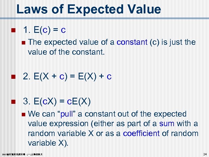
Laws of Expected Value n 1. E(c) = c n The expected value of a constant (c) is just the value of the constant. n 2. E(X + c) = E(X) + c n 3. E(c. X) = c. E(X) n We can “pull” a constant out of the expected value expression (either as part of a sum with a random variable X or as a coefficient of random variable X). 2007會計資訊系統計學 (一)上課投影片 24
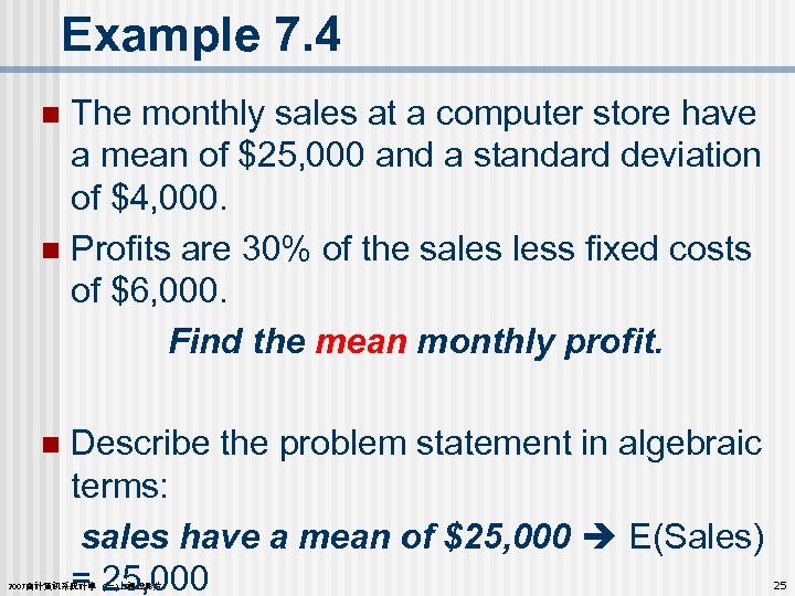
Example 7. 4 The monthly sales at a computer store have a mean of $25, 000 and a standard deviation of $4, 000. n Profits are 30% of the sales less fixed costs of $6, 000. Find the mean monthly profit. n n Describe the problem statement in algebraic terms: sales have a mean of $25, 000 E(Sales) = 25, 000 2007會計資訊系統計學 (一)上課投影片 25
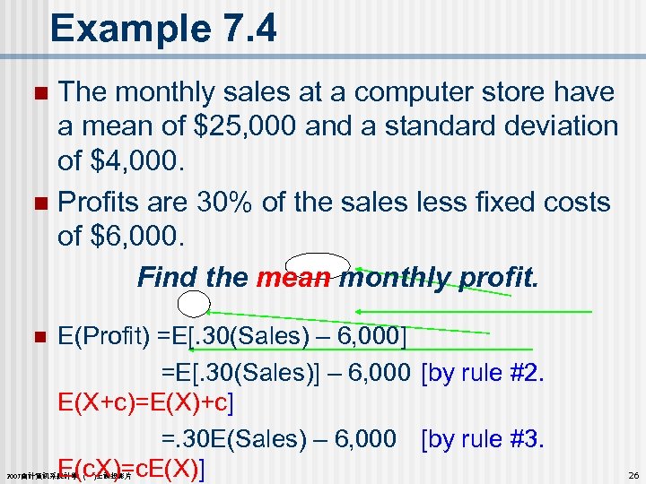
Example 7. 4 The monthly sales at a computer store have a mean of $25, 000 and a standard deviation of $4, 000. n Profits are 30% of the sales less fixed costs of $6, 000. Find the mean monthly profit. n n E(Profit) =E[. 30(Sales) – 6, 000] =E[. 30(Sales)] – 6, 000 [by rule #2. E(X+c)=E(X)+c] =. 30 E(Sales) – 6, 000 [by rule #3. E(c. X)=c. E(X)] 2007會計資訊系統計學 (一)上課投影片 26
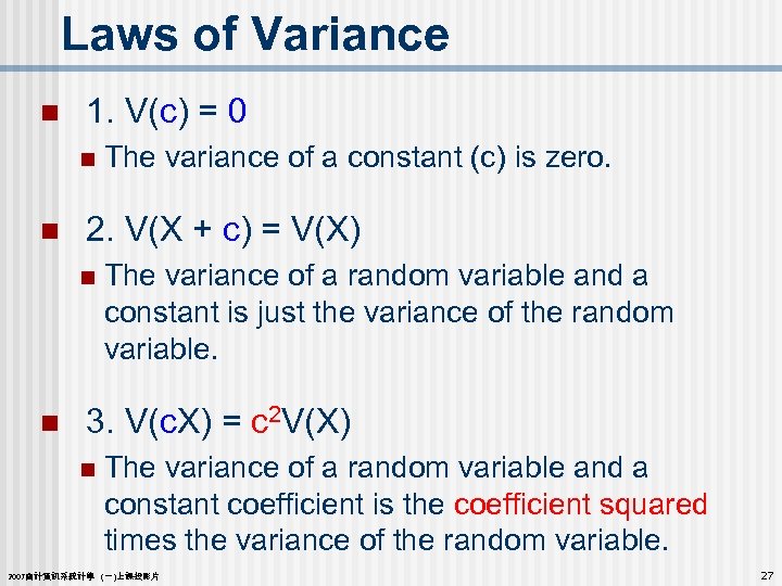
Laws of Variance n 1. V(c) = 0 n n 2. V(X + c) = V(X) n n The variance of a constant (c) is zero. The variance of a random variable and a constant is just the variance of the random variable. 3. V(c. X) = c 2 V(X) n The variance of a random variable and a constant coefficient is the coefficient squared times the variance of the random variable. 2007會計資訊系統計學 (一)上課投影片 27
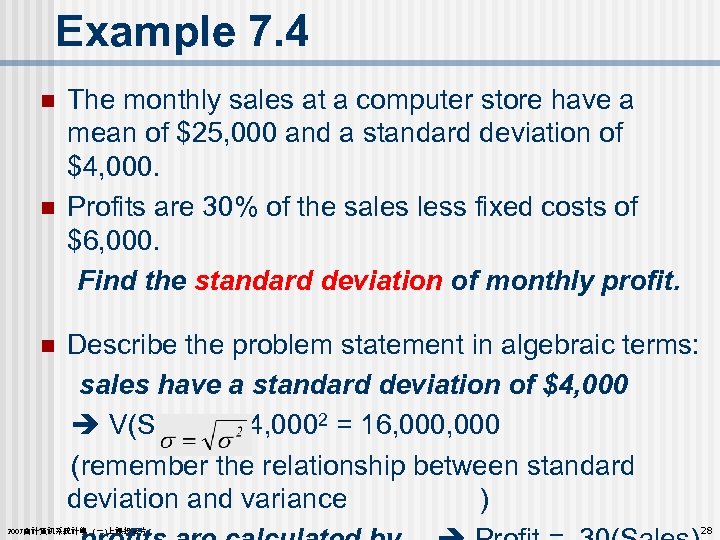
Example 7. 4 n n The monthly sales at a computer store have a mean of $25, 000 and a standard deviation of $4, 000. Profits are 30% of the sales less fixed costs of $6, 000. Find the standard deviation of monthly profit. Describe the problem statement in algebraic terms: sales have a standard deviation of $4, 000 V(Sales) = 4, 0002 = 16, 000 (remember the relationship between standard deviation and variance ) n 2007會計資訊系統計學 (一)上課投影片 28
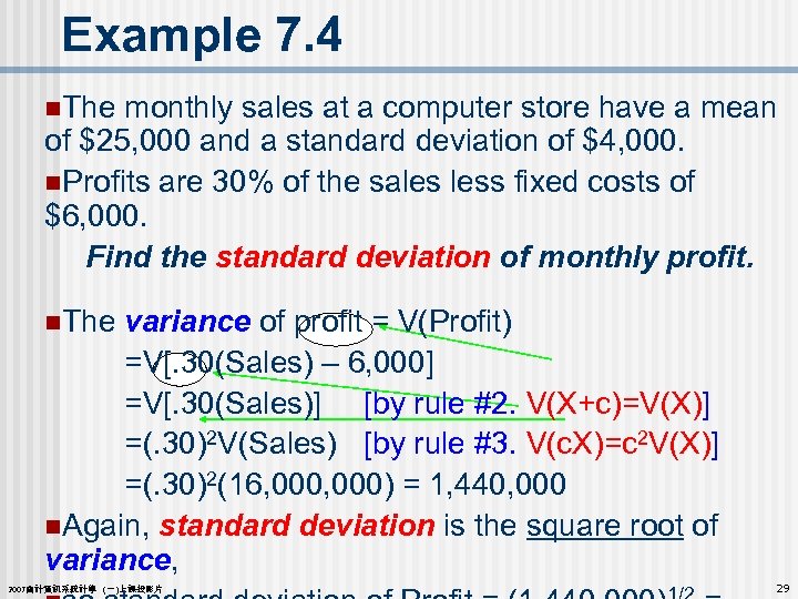
Example 7. 4 n. The monthly sales at a computer store have a mean of $25, 000 and a standard deviation of $4, 000. n. Profits are 30% of the sales less fixed costs of $6, 000. Find the standard deviation of monthly profit. n. The variance of profit = V(Profit) =V[. 30(Sales) – 6, 000] =V[. 30(Sales)] [by rule #2. V(X+c)=V(X)] =(. 30)2 V(Sales) [by rule #3. V(c. X)=c 2 V(X)] =(. 30)2(16, 000) = 1, 440, 000 n. Again, standard deviation is the square root of variance, 2007會計資訊系統計學 (一)上課投影片 29
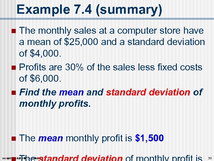
Example 7. 4 (summary) The monthly sales at a computer store have a mean of $25, 000 and a standard deviation of $4, 000. n Profits are 30% of the sales less fixed costs of $6, 000. n Find the mean and standard deviation of monthly profits. n n The mean monthly profit is $1, 500 2007會計資訊系統計學 (一)上課投影片 30
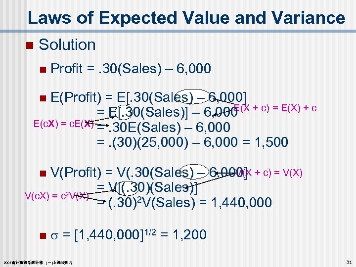
Laws of Expected Value and Variance n Solution n Profit =. 30(Sales) – 6, 000 E(Profit) = E[. 30(Sales) – 6, 000] E(X + c) = E(X) + c = E[. 30(Sales)] – 6, 000 E(c. X) = c. E(X) =. 30 E(Sales) – 6, 000 =. (30)(25, 000) – 6, 000 = 1, 500 n V(X + c) = V(X) V(Profit) = V(. 30(Sales) – 6, 000] = V[(. 30)(Sales)] V(c. X) = c 2 V(X) = (. 30)2 V(Sales) = 1, 440, 000 n n s = [1, 440, 000]1/2 = 1, 2007會計資訊系統計學 (一)上課投影片 31
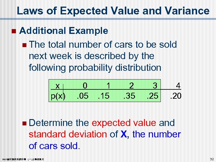
Laws of Expected Value and Variance n Additional Example n The total number of cars to be sold next week is described by the following probability distribution x 0 1 2 3 4 p(x) . 05 . 15 . 35 . 20 n Determine the expected value and standard deviation of X, the number of cars sold. 2007會計資訊系統計學 (一)上課投影片 32
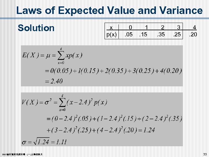
Laws of Expected Value and Variance Solution 2007會計資訊系統計學 (一)上課投影片 x 0 1 2 3 4 p(x) . 05 . 15 . 35 . 20 33
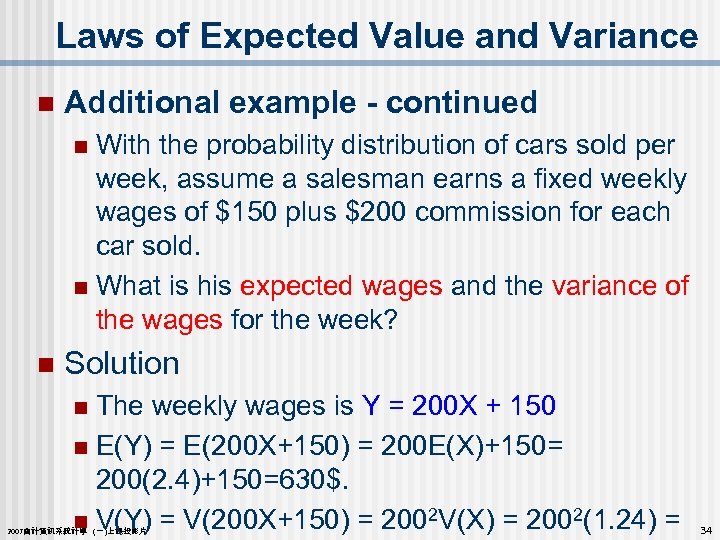
Laws of Expected Value and Variance n Additional example - continued With the probability distribution of cars sold per week, assume a salesman earns a fixed weekly wages of $150 plus $200 commission for each car sold. n What is his expected wages and the variance of the wages for the week? n n Solution The weekly wages is Y = 200 X + 150 n E(Y) = E(200 X+150) = 200 E(X)+150= 200(2. 4)+150=630$. n V(Y) = V(200 X+150) = 2002 V(X) = 2002(1. 24) = n 2007會計資訊系統計學 (一)上課投影片 34
7. 2 Bivariate Distributions n n n Up to now, we have looked at univariate distributions, i. e. probability distributions in one variable. As you might guess, bivariate distributions(二元 分配) are probabilities of combinations of two variables. The bivariate (or joint) distribution is used when the relationship between two random variables is studied. A joint probability distribution of X and Y is a table or formula that lists the joint probabilities for all pairs of values x and y, and is denoted P(x, y). The probability that X assumes the value x, and Y 2007會計資訊系統計學 (一)上課投影片 35
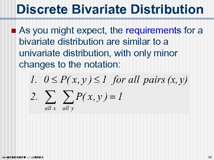
Discrete Bivariate Distribution n As you might expect, the requirements for a bivariate distribution are similar to a univariate distribution, with only minor changes to the notation: 2007會計資訊系統計學 (一)上課投影片 36
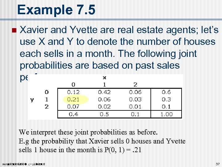
Example 7. 5 n Xavier and Yvette are real estate agents; let’s use X and Y to denote the number of houses each sells in a month. The following joint probabilities are based on past sales performance: We interpret these joint probabilities as before. E. g the probability that Xavier sells 0 houses and Yvette sells 1 house in the month is P(0, 1) =. 21 2007會計資訊系統計學 (一)上課投影片 37
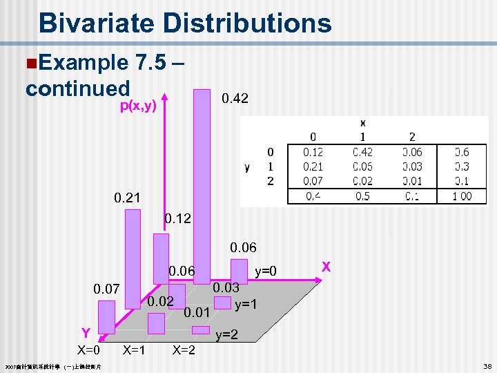
Bivariate Distributions n. Example 7. 5 – continued 0. 42 p(x, y) 0. 21 0. 12 0. 06 0. 07 0. 02 0. 01 Y X=0 2007會計資訊系統計學 (一)上課投影片 y=0 X 0. 03 y=1 y=2 X=1 X=2 38
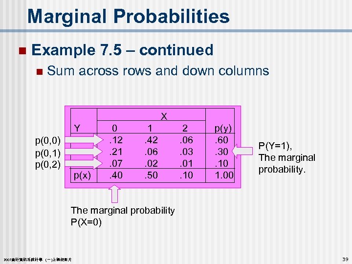
Marginal Probabilities n Example 7. 5 – continued n Sum across rows and down columns X Y 0 1 0. 12. 42 1. 21. 06 2. 07. 02 p(x). 40. 50 p(0, 0) p(0, 1) p(0, 2) 2. 06. 03. 01. 10 p(y). 60. 30. 10 1. 00 P(Y=1), The marginal probability P(X=0) 2007會計資訊系統計學 (一)上課投影片 39
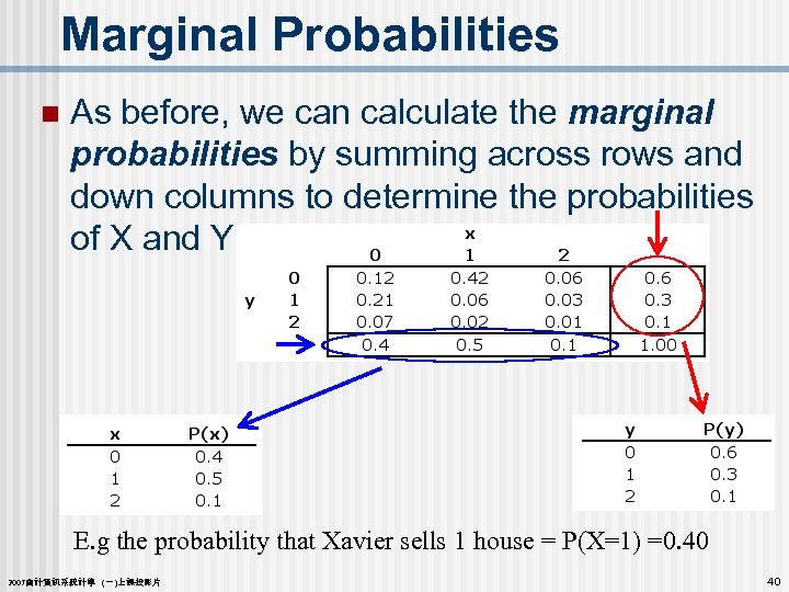
Marginal Probabilities n As before, we can calculate the marginal probabilities by summing across rows and down columns to determine the probabilities of X and Y individually: E. g the probability that Xavier sells 1 house = P(X=1) =0. 40 2007會計資訊系統計學 (一)上課投影片 40
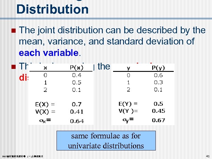
Distribution The joint distribution can be described by the mean, variance, and standard deviation of each variable. n This is done using the marginal distributions. n same formulae as for univariate distributions 2007會計資訊系統計學 (一)上課投影片 41
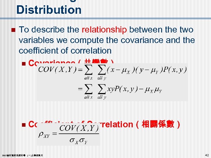
Distribution n To describe the relationship between the two variables we compute the covariance and the coefficient of correlation n Covariance(共變數) n Coefficient of Correlation(相關係數) 2007會計資訊系統計學 (一)上課投影片 42
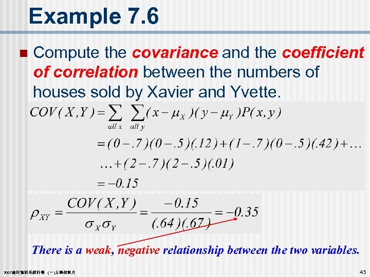
Example 7. 6 n Compute the covariance and the coefficient of correlation between the numbers of houses sold by Xavier and Yvette. There is a weak, negative relationship between the two variables. 2007會計資訊系統計學 (一)上課投影片 43
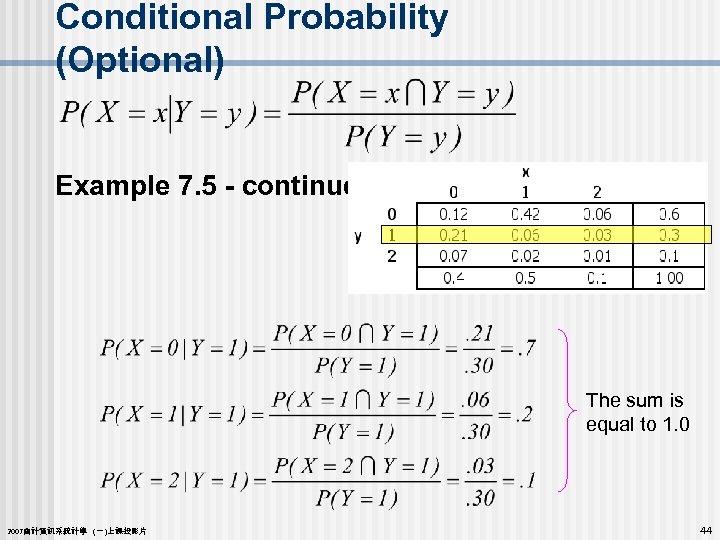
Conditional Probability (Optional) Example 7. 5 - continued The sum is equal to 1. 0 2007會計資訊系統計學 (一)上課投影片 44
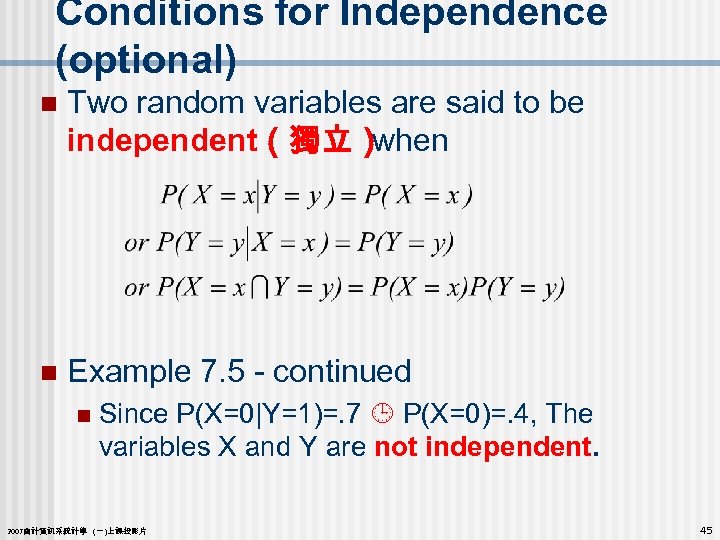
Conditions for Independence (optional) n Two random variables are said to be independent(獨立) when n Example 7. 5 - continued n Since P(X=0|Y=1)=. 7 P(X=0)=. 4, The variables X and Y are not independent. 2007會計資訊系統計學 (一)上課投影片 45
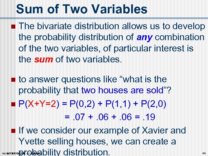
Sum of Two Variables n The bivariate distribution allows us to develop the probability distribution of any combination of the two variables, of particular interest is the sum of two variables. to answer questions like “what is the probability that two houses are sold”? n P(X+Y=2) = P(0, 2) + P(1, 1) + P(2, 0) =. 07 +. 06 =. 19 n If we consider our example of Xavier and Yvette selling houses, we can create a probability distribution. n 2007會計資訊系統計學 (一)上課投影片 46
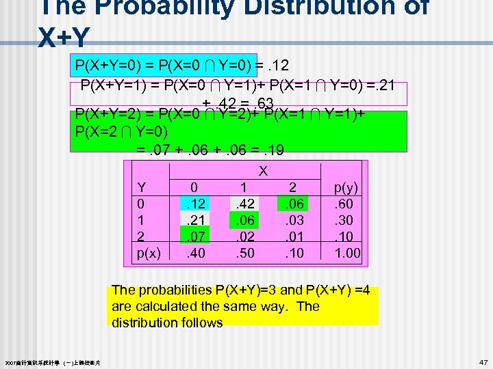
The Probability Distribution of X+Y P(X+Y=0) = P(X=0 Y=0) =. 12 P(X+Y=1) = P(X=0 Y=1)+ P(X=1 Y=0) =. 21 +. 42 =. 63 P(X+Y=2) = P(X=0 Y=2)+ P(X=1 Y=1)+ P(X=2 Y=0) =. 07 +. 06 =. 19 X Y 0 1 0. 12. 42 1. 21. 06 2. 07. 02 p(x). 40. 50 2. 06. 03. 01. 10 p(y). 60. 30. 10 1. 00 The probabilities P(X+Y)=3 and P(X+Y) =4 are calculated the same way. The distribution follows 2007會計資訊系統計學 (一)上課投影片 47
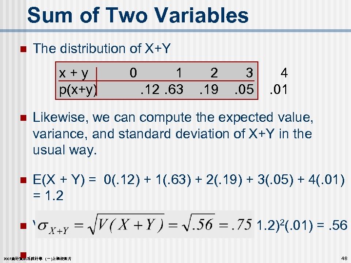
Sum of Two Variables n The distribution of X+Y x + y 0 1 p(x+y) . 12. 63 2. 19 3. 05 4. 01 n Likewise, we can compute the expected value, variance, and standard deviation of X+Y in the usual way. n E(X + Y) = 0(. 12) + 1(. 63) + 2(. 19) + 3(. 05) + 4(. 01) = 1. 2 n V(X + Y) = (0 – 1. 2)2(. 12) + … + (4 – 1. 2)2(. 01) =. 56 n 2007會計資訊系統計學 (一)上課投影片 48
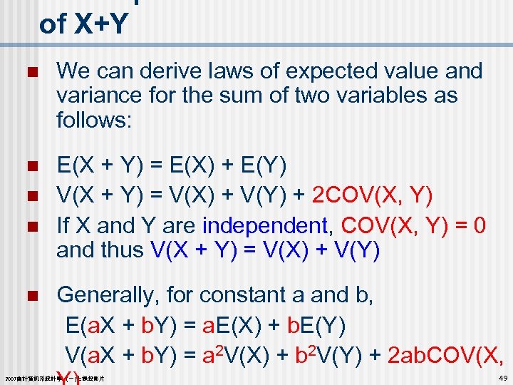
of X+Y n We can derive laws of expected value and variance for the sum of two variables as follows: n E(X + Y) = E(X) + E(Y) V(X + Y) = V(X) + V(Y) + 2 COV(X, Y) If X and Y are independent, COV(X, Y) = 0 and thus V(X + Y) = V(X) + V(Y) n n Generally, for constant a and b, E(a. X + b. Y) = a. E(X) + b. E(Y) V(a. X + b. Y) = a 2 V(X) + b 2 V(Y) + 2 ab. COV(X, n 2007會計資訊系統計學 (一)上課投影片 49
7. 4 Binomial Distribution § The binomial distribution (二項分配) is the probability distribution that results from doing a “binomial experiment(二項實驗) ”. Binomial experiments have the following properties: § Fixed number of trials, represented as n. § Each trial has two possible outcomes, a “success” and a “failure”. § P(success)=p (and thus: P(failure)=1–p), for all trials. § The trials are independent, which means that 2007會計資訊系統計學 (一)上課投影片 50
Success and Failure n …are just labels for a binomial experiment, there is no value judgment implied. n For example a coin flip will result in either heads or tails. If we define “heads” as success then necessarily “tails” is considered a failure (inasmuch as we attempting to have the coin lands heads up). n Other binomial experiment notions: n n A coin flipped results in heads or tails An election candidate wins or loses An employee is male or female A car uses 87 octane gasoline, or another gasoline. 2007會計資訊系統計學 (一)上課投影片 51

Binomial Random Variable n The random variable of a binomial experiment is defined as the number of successes in the n trials, and is called the binomial random variable(二項 隨機變數). n E. g. flip a fair coin 10 times. 1) Fixed number of trials n=10 2) Each trial has two possible outcomes {heads (success), tails (failure)} 3) P(success)= 0. 50; P(failure)=1– 0. 50 = 0. 50 4) The trials are independent (i. e. the outcome of heads on the first flip will have no impact on subsequent coin flips). n Hence flipping a coin ten times is a binomial 2007會計資訊系統計學 (一)上課投影片 52
Binomial Random Variable n The binomial random variable counts the number of successes in n trials of the binomial experiment. It can take on values from 0, 1, 2, …, n. Thus, its a discrete random variable. 2007會計資訊系統計學 (一)上課投影片 53
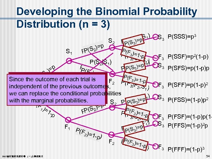
Developing the Binomial Probability Distribution (n = 3) S 1 )=p S|S 1) 2 P( P(S 2 ) |S 2, S 1 P(S 3 )=p S 3 P(SSS)=p 3 P(F | 1 -p 3 S 2 , S ) S , p 11) F P( 3| 2 P(SS 3)= F 3 P(SSF)=p 2(1 -p) S 3 P(SFS)=p(1 -p)p P(S 3 P(F 3 )= P(S 2|S 1) P(F p P(F |S ) )= 2) 1 1 2 =1(S p P(F ) P Since the outcome of each trial is F 2 P(F 3 =1 -p 3 |F 2 , S independent of the previous outcomes, 1) we can replace the conditional probabilities ) |S)2, F 1 =p with the marginal probabilities. SS P( S 2 P(P(3 3 F p 1 )= F=) P (S|2) 1 P 1 -p P(S 2 P(F(F 3 )=1 -p 3 |S 2 , F 1) , F ) |F=p 1 2 F 1 (S 3 PP(S 3) P(F (F P 2 )=1 F ) 2| 1 p F 2 PPF 3 F 1 ( (F | )= 3 2 , F p) 1 2007會計資訊系統計學 (一)上課投影片 F 3 P(SFF)=p(1 -p)2 S 3 P(FSS)=(1 -p)p 2 F 3 P(FSF)=(1 -p)p(1 S 3 P(FFS)=(1 -p)2 p F 3 P(FFF)=(1 -p)3 54
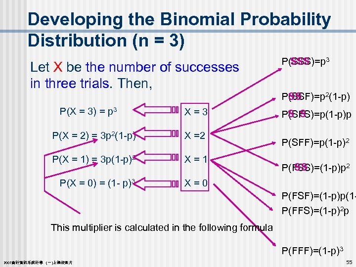
Developing the Binomial Probability Distribution (n = 3) Let X be the number of successes in three trials. Then, P(X = 3) = p 3 X = 3 P(X = 2) = 3 p 2(1 -p) X =2 P(X = 1) = 3 p(1 -p)2 X = 1 P(X = 0) = (1 - p)3 P(SSS)=p 3 SSS P(SSF)=p 2(1 -p) SS S S P(SFS)=p(1 -p)p X = 0 P(SFF)=p(1 -p)2 SS P(FSS)=(1 -p)p 2 P(FSF)=(1 -p)p(1 P(FFS)=(1 -p)2 p This multiplier is calculated in the following formula P(FFF)=(1 -p)3 2007會計資訊系統計學 (一)上課投影片 55
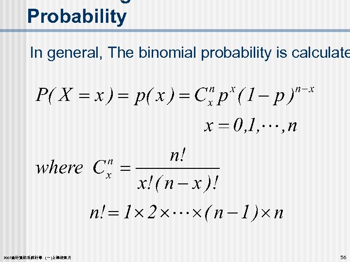
Probability In general, The binomial probability is calculate 2007會計資訊系統計學 (一)上課投影片 56
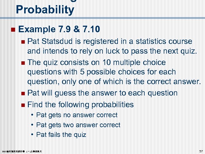
Probability n Example 7. 9 & 7. 10 Pat Statsdud is registered in a statistics course and intends to rely on luck to pass the next quiz. n The quiz consists on 10 multiple choice questions with 5 possible choices for each question, only one of which is the correct answer. n Pat will guess the answer to each question n Find the following probabilities n • Pat gets no answer correct • Pat gets two answer correct • Pat fails the quiz 2007會計資訊系統計學 (一)上課投影片 57
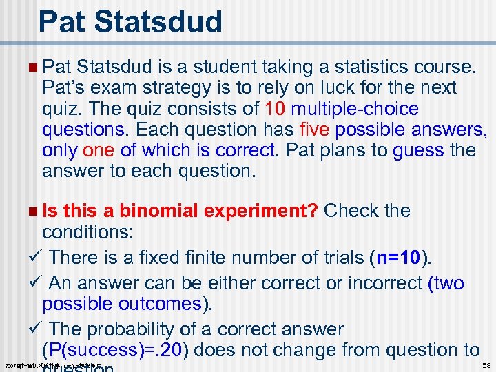
Pat Statsdud n Pat Statsdud is a student taking a statistics course. Pat’s exam strategy is to rely on luck for the next quiz. The quiz consists of 10 multiple-choice questions. Each question has five possible answers, only one of which is correct. Pat plans to guess the answer to each question. n Is this a binomial experiment? Check the conditions: There is a fixed finite number of trials (n=10). An answer can be either correct or incorrect (two possible outcomes). The probability of a correct answer (P(success)=. 20) does not change from question to 2007會計資訊系統計學 (一)上課投影片 58
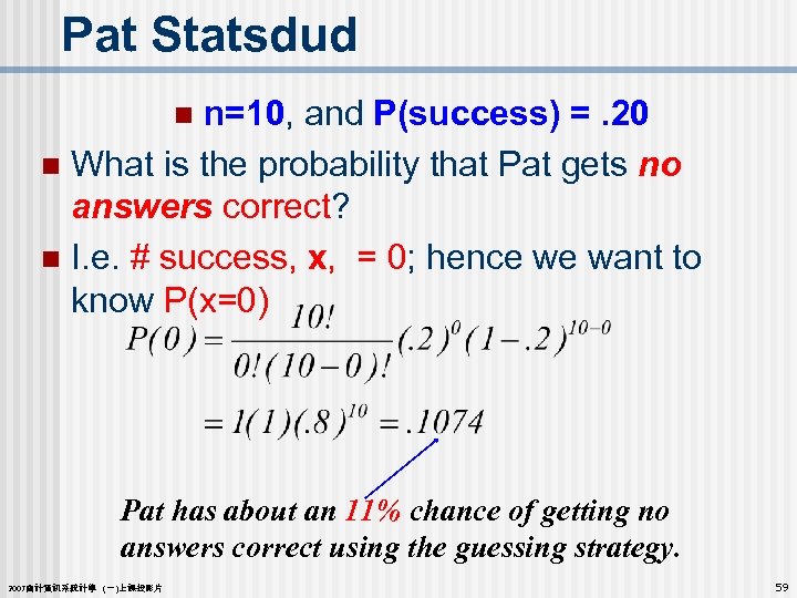
Pat Statsdud n=10, and P(success) =. 20 n What is the probability that Pat gets no answers correct? n I. e. # success, x, = 0; hence we want to know P(x=0) n Pat has about an 11% chance of getting no answers correct using the guessing strategy. 2007會計資訊系統計學 (一)上課投影片 59
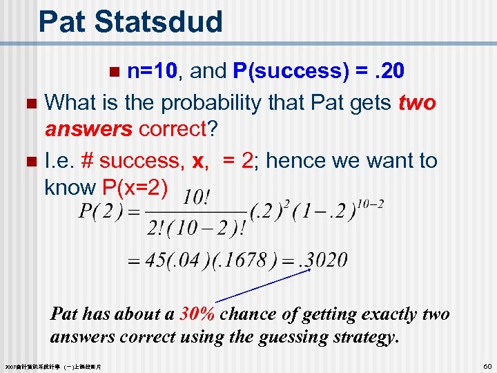
Pat Statsdud n=10, and P(success) =. 20 n What is the probability that Pat gets two answers correct? n I. e. # success, x, = 2; hence we want to know P(x=2) n Pat has about a 30% chance of getting exactly two answers correct using the guessing strategy. 2007會計資訊系統計學 (一)上課投影片 60
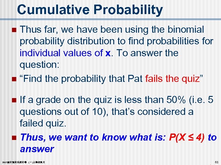
Cumulative Probability Thus far, we have been using the binomial probability distribution to find probabilities for individual values of x. To answer the question: n “Find the probability that Pat fails the quiz” n If a grade on the quiz is less than 50% (i. e. 5 questions out of 10), that’s considered a failed quiz. n Thus, we want to know what is: P(X ≤ 4) to answer n 2007會計資訊系統計學 (一)上課投影片 61
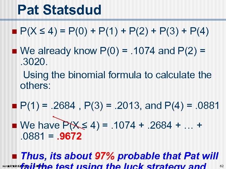
Pat Statsdud n P(X ≤ 4) = P(0) + P(1) + P(2) + P(3) + P(4) We already know P(0) =. 1074 and P(2) = . 3020. Using the binomial formula to calculate the others: n n P(1) =. 2684 , P(3) =. 2013, and P(4) =. 0881 n We have P(X ≤ 4) =. 1074 +. 2684 + … + . 0881 =. 9672 n Thus, its about 97% probable that Pat will 2007會計資訊系統計學 (一)上課投影片 62
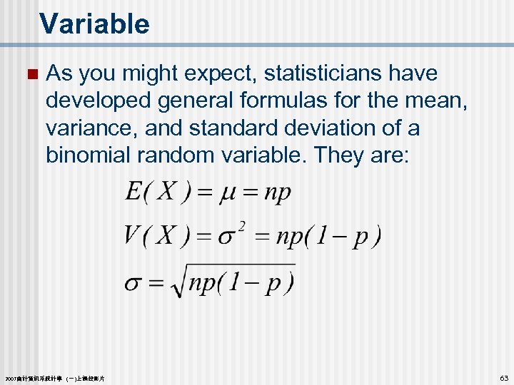
Variable n As you might expect, statisticians have developed general formulas for the mean, variance, and standard deviation of a binomial random variable. They are: 2007會計資訊系統計學 (一)上課投影片 63
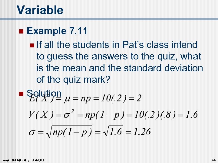
Variable Example 7. 11 n If all the students in Pat’s class intend to guess the answers to the quiz, what is the mean and the standard deviation of the quiz mark? n Solution n 2007會計資訊系統計學 (一)上課投影片 64
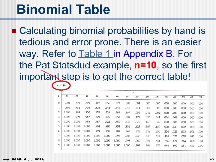
Binomial Table n Calculating binomial probabilities by hand is tedious and error prone. There is an easier way. Refer to Table 1 in Appendix B. For the Pat Statsdud example, n=10, so the first important step is to get the correct table! 2007會計資訊系統計學 (一)上課投影片 65
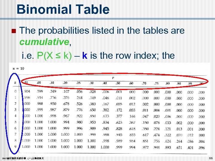
Binomial Table The probabilities listed in the tables are cumulative, i. e. P(X ≤ k) – k is the row index; the columns of the table are organized by P(success) = p n 2007會計資訊系統計學 (一)上課投影片 66
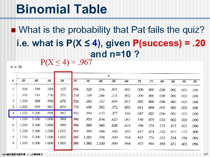
Binomial Table n What is the probability that Pat fails the quiz? i. e. what is P(X ≤ 4), given P(success) =. 20 and n=10 ? P(X ≤ 4) =. 967 2007會計資訊系統計學 (一)上課投影片 67
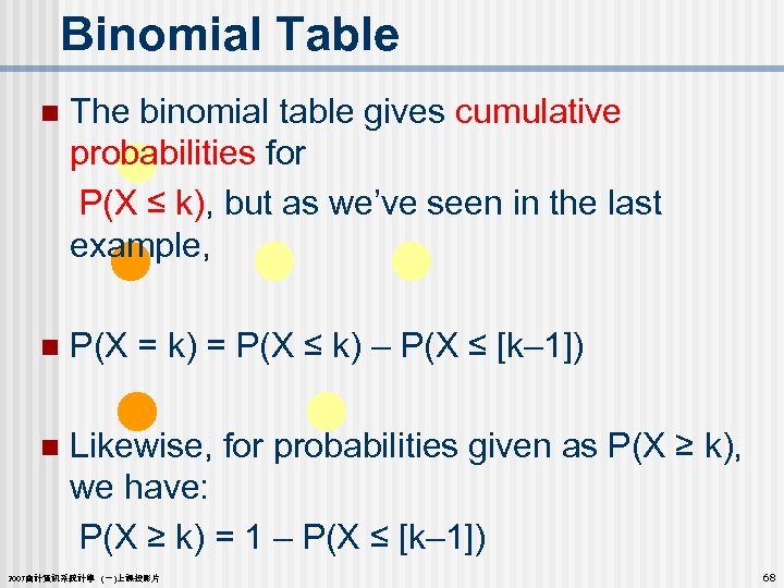
Binomial Table The binomial table gives cumulative probabilities for P(X ≤ k), but as we’ve seen in the last example, n n P(X = k) = P(X ≤ k) – P(X ≤ [k– 1]) Likewise, for probabilities given as P(X ≥ k), we have: P(X ≥ k) = 1 – P(X ≤ [k– 1]) n 2007會計資訊系統計學 (一)上課投影片 68
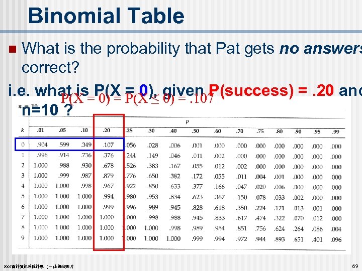
Binomial Table What is the probability that Pat gets no answers correct? i. e. what is P(X = 0), given P(success) =. 20 and P(X = 0) = P(X ≤ 0) =. 107 n=10 ? n 2007會計資訊系統計學 (一)上課投影片 69
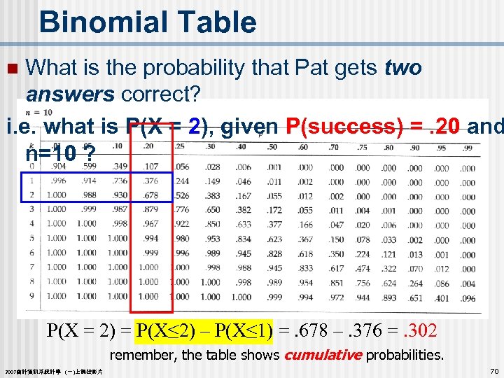
Binomial Table What is the probability that Pat gets two answers correct? i. e. what is P(X = 2), given P(success) =. 20 and n=10 ? n P(X = 2) = P(X≤ 2) – P(X≤ 1) =. 678 –. 376 =. 302 remember, the table shows cumulative probabilities. 2007會計資訊系統計學 (一)上課投影片 70
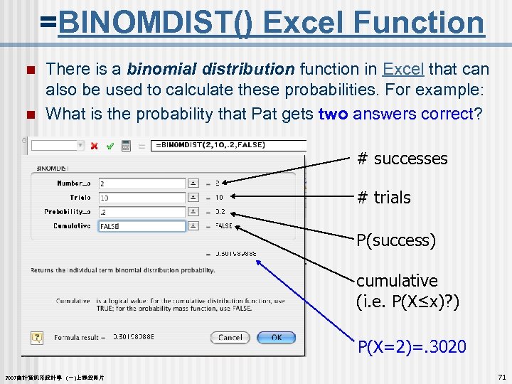
=BINOMDIST() Excel Function n n There is a binomial distribution function in Excel that can also be used to calculate these probabilities. For example: What is the probability that Pat gets two answers correct? # successes # trials P(success) cumulative (i. e. P(X≤x)? ) P(X=2)=. 3020 2007會計資訊系統計學 (一)上課投影片 71
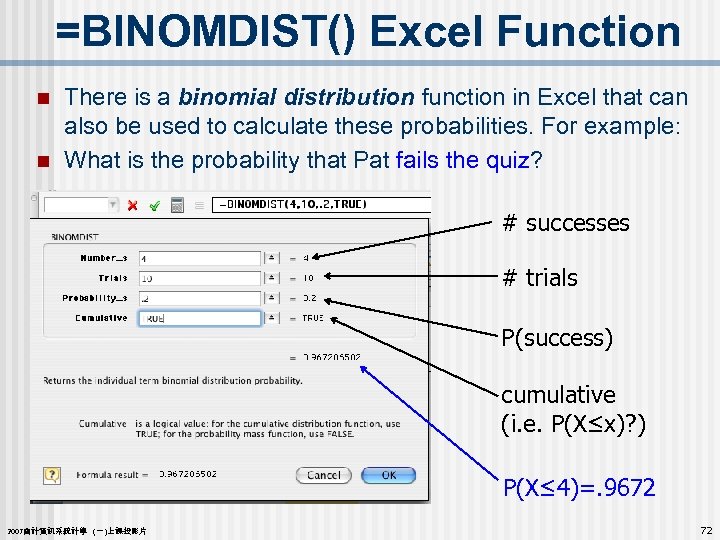
=BINOMDIST() Excel Function n n There is a binomial distribution function in Excel that can also be used to calculate these probabilities. For example: What is the probability that Pat fails the quiz? # successes # trials P(success) cumulative (i. e. P(X≤x)? ) P(X≤ 4)=. 9672 2007會計資訊系統計學 (一)上課投影片 72
Binomial Distribution n Additional Example Records show that 30% of the customers in a shoe store make their payments using a credit card. n This morning 20 customers purchased shoes. n Use Table 1 of Appendix B to answer some questions stated in the next slide. n This is a binomial experiment with n=20 and p=. 30. n Let X be the number of customers who use a credit card. n 2007會計資訊系統計學 (一)上課投影片 73
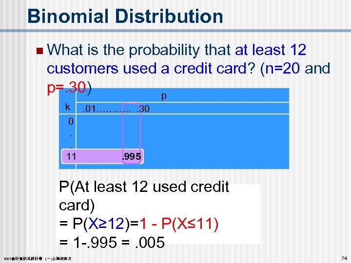
Binomial Distribution n What is the probability that at least 12 customers used a credit card? (n=20 and p=. 30) p k 0. . 11 . 01………. . . 30 . 995 P(At least 12 used credit card) = P(X≥ 12)=1 - P(X≤ 11) = 1 -. 995 =. 005 2007會計資訊系統計學 (一)上課投影片 74
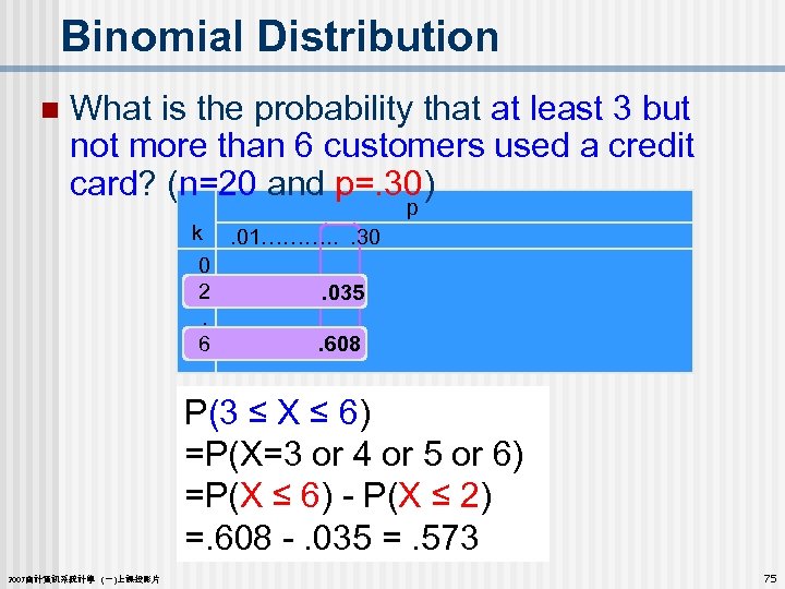
Binomial Distribution n What is the probability that at least 3 but not more than 6 customers used a credit card? (n=20 and p=. 30) p k 0 2. 6 . 01………. . . 30. 035. 608 P(3 ≤ X ≤ 6) =P(X=3 or 4 or 5 or 6) =P(X ≤ 6) - P(X ≤ 2) =. 608 -. 035 =. 573 2007會計資訊系統計學 (一)上課投影片 75
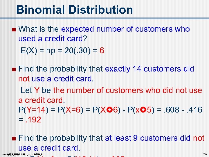
Binomial Distribution What is the expected number of customers who used a credit card? E(X) = np = 20(. 30) = 6 n Find the probability that exactly 14 customers did not use a credit card. Let Y be the number of customers who did not use a credit card. P(Y=14) = P(X=6) = P(X 6) - P(x 5) =. 608 -. 416 =. 192 n n Find the probability that at least 9 customers did not use a credit card. 2007會計資訊系統計學 (一)上課投影片 76
7. 5 Poisson Distribution The Poisson distribution, named for Simeon Poisson, is a discrete probability distribution n It refers to the number of events (a. k. a. successes) within a specific time period or a specific region of space. n 2007會計資訊系統計學 (一)上課投影片 77
Distribution The number of errors a typist makes per page. n The number of flaws in a bolt of cloth. n The number of telephone calls received by a switchboard in an hour. n The number of customers entering a service station per day. n The number of cars arriving at a service station in a week. n The number of accidents in 1 day on a particular stretch of highway. (The interval is defined by both time, 1 day, and space, the n 2007會計資訊系統計學 (一)上課投影片 78
Properties of the Poisson Experiment n Like a binomial experiment, a Poisson experiment has four defining characteristic properties: The number of successes (events) that occur in any interval is independent of the number of successes that occur in any other interval. n The probability of a success in an interval is • the same for all intervals of the same size, • proportional to the size of the interval. n The probability that two or more successes will occur in an interval approaches 0 as the interval becomes smaller. n 2007會計資訊系統計學 (一)上課投影片 79
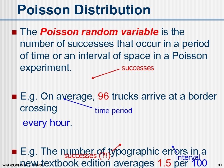
Poisson Distribution n The Poisson random variable is the number of successes that occur in a period of time or an interval of space in a Poisson successes experiment. E. g. On average, 96 trucks arrive at a border crossing time period every hour. n n E. g. The number of typographic errors in a successes (? !) interval new textbook edition averages 1. 5 per 100 2007會計資訊系統計學 (一)上課投影片 80
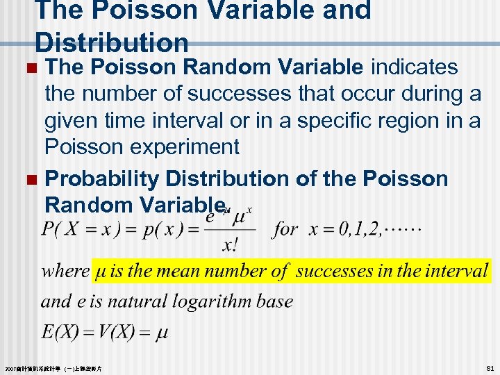
The Poisson Variable and Distribution The Poisson Random Variable indicates the number of successes that occur during a given time interval or in a specific region in a Poisson experiment n Probability Distribution of the Poisson Random Variable. n 2007會計資訊系統計學 (一)上課投影片 81
Poisson Distribution n As mentioned on the Poisson experiment slide: n The probability of a success is proportional to the size of the interval n Thus, knowing an error rate of 1. 5 typos per 100 pages, we can determine a mean value for a 400 page book as: =1. 5(4) = 6 typos / 400 pages. 2007會計資訊系統計學 (一)上課投影片 82
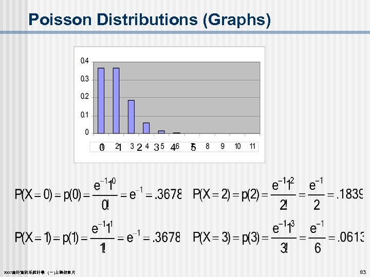
Poisson Distributions (Graphs) 0 1 2 3 4 5 2007會計資訊系統計學 (一)上課投影片 83
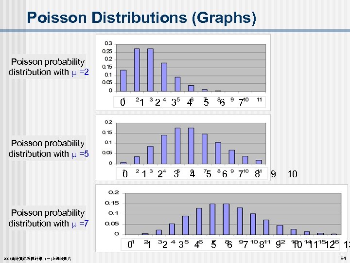
Poisson Distributions (Graphs) Poisson probability distribution with =2 0 1 2 3 4 5 6 7 Poisson probability distribution with =5 0 1 2 3 4 5 6 7 8 9 10 Poisson probability distribution with =7 0 1 2 3 4 5 6 7 8 9 10 11 12 13 2007會計資訊系統計學 (一)上課投影片 84
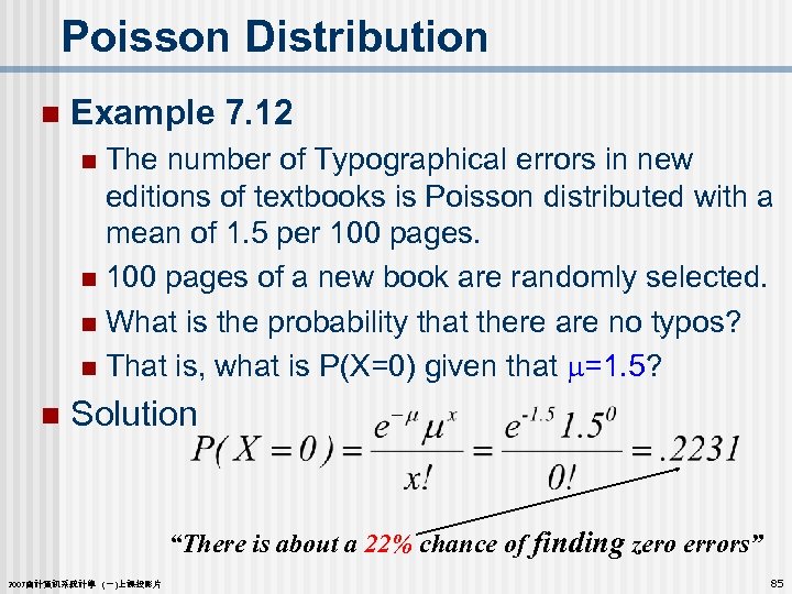
Poisson Distribution n Example 7. 12 The number of Typographical errors in new editions of textbooks is Poisson distributed with a mean of 1. 5 per 100 pages. n 100 pages of a new book are randomly selected. n What is the probability that there are no typos? n That is, what is P(X=0) given that =1. 5? n n Solution “There is about a 22% chance of finding zero errors” 2007會計資訊系統計學 (一)上課投影片 85
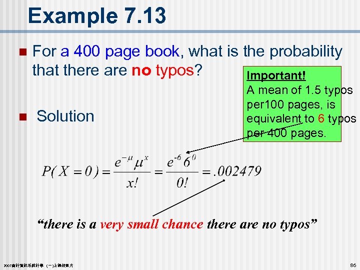
Example 7. 13 n n For a 400 page book, what is the probability that there are no typos? Important! Solution A mean of 1. 5 typos per 100 pages, is equivalent to 6 typos per 400 pages. “there is a very small chance there are no typos” 2007會計資訊系統計學 (一)上課投影片 86
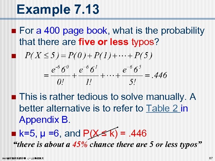
Example 7. 13 For a 400 page book, what is the probability that there are five or less typos? n n This is rather tedious to solve manually. A better alternative is to refer to Table 2 in Appendix B. n k=5, μ =6, and P(X ≤ k) =. 446 n “there is about a 45% chance there are 5 or less typos” 2007會計資訊系統計學 (一)上課投影片 87
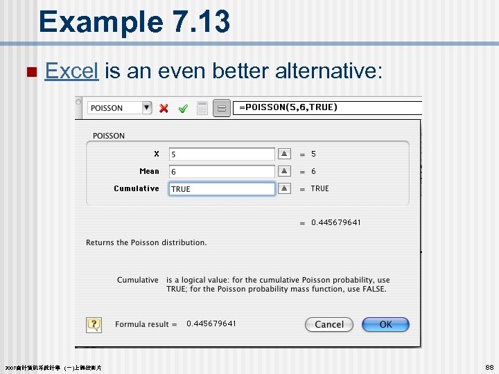
Example 7. 13 n Excel is an even better alternative: 2007會計資訊系統計學 (一)上課投影片 88
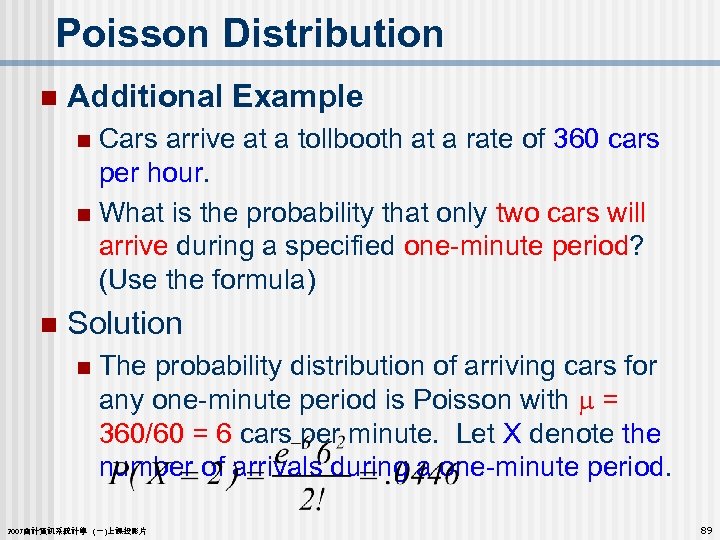
Poisson Distribution n Additional Example Cars arrive at a tollbooth at a rate of 360 cars per hour. n What is the probability that only two cars will arrive during a specified one-minute period? (Use the formula) n n Solution n The probability distribution of arriving cars for any one-minute period is Poisson with = 360/60 = 6 cars per minute. Let X denote the number of arrivals during a one-minute period. 2007會計資訊系統計學 (一)上課投影片 89
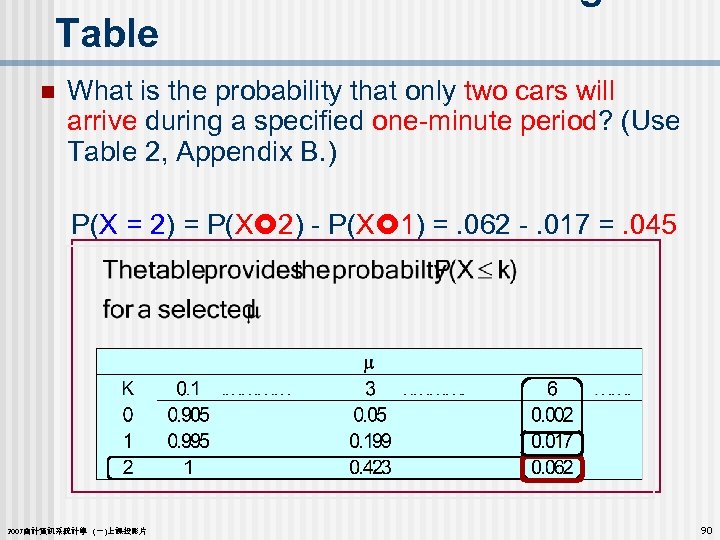
Table n What is the probability that only two cars will arrive during a specified one-minute period? (Use Table 2, Appendix B. ) P(X = 2) = P(X 2) - P(X 1) =. 062 -. 017 =. 045 2007會計資訊系統計學 (一)上課投影片 90
Table n What is the probability that at least four cars will arrive during a one-minute period? (Use table 2 , Appendix B) P(X 4) = 1 - P(X 3) = 1 -. 151 =. 849 2007會計資訊系統計學 (一)上課投影片 91
Poisson Approximation of the Binomial (Optional) n Example A warehouse has a policy of examining 50 sunglasses from each incoming lot, and accepting the lot only if there are no more than two defective pairs. n What is the probability of a lot being accepted if, in fact, 2% of the sunglasses are defective? n n Solution This is a binomial experiment with n = 50, p = . 02. n Tables for n = 50 are not available; n p<. 05; thus, a Poisson approximation is appropriate [ = (50)(. 02) =1] n 2007會計資訊系統計學 (一)上課投影片 92
45b0e33d16e0122b2253d2b35a8bb811.ppt