Chapter 6 Using Data Structures 1 Using

Chapter 6: Using Data Structures 1

Using Data Structures Records u Lists u Association Lists u Binary Trees u Hierarchical Modelling u Tree Layout u 2

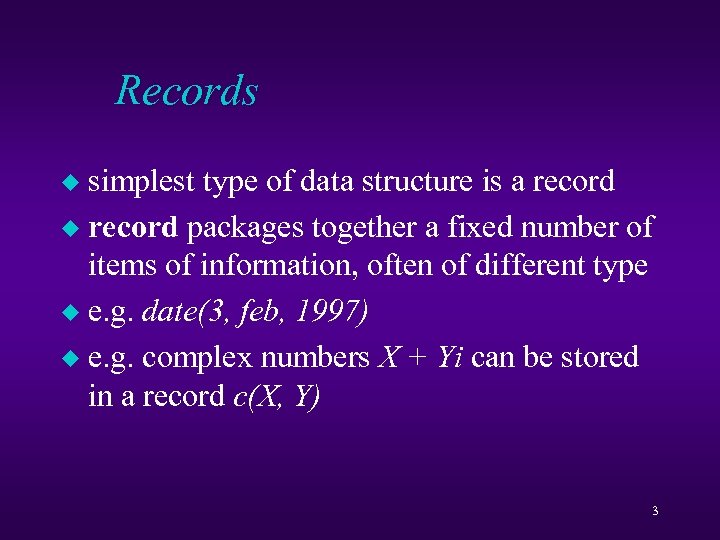Records simplest type of data structure is a record u record packages together a fixed number of items of information, often of different type u e. g. date(3, feb, 1997) u e. g. complex numbers X + Yi can be stored in a record c(X, Y) u 3

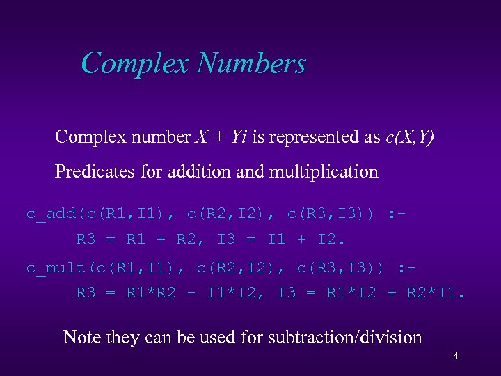Complex Numbers Complex number X + Yi is represented as c(X, Y) Predicates for addition and multiplication c_add(c(R 1, I 1), c(R 2, I 2), c(R 3, I 3)) : R 3 = R 1 + R 2, I 3 = I 1 + I 2. c_mult(c(R 1, I 1), c(R 2, I 2), c(R 3, I 3)) : R 3 = R 1*R 2 - I 1*I 2, I 3 = R 1*I 2 + R 2*I 1. Note they can be used for subtraction/division 4

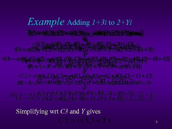Example Adding 1+3 i to 2+Yi Simplifying wrt C 3 and Y gives 5

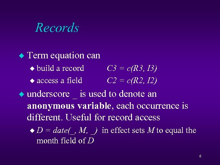Records u Term equation can u build a record u access a field u C 3 = c(R 3, I 3) C 2 = c(R 2, I 2) underscore _ is used to denote an anonymous variable, each occurrence is different. Useful for record access u. D = date(_, M, _) in effect sets M to equal the month field of D 6

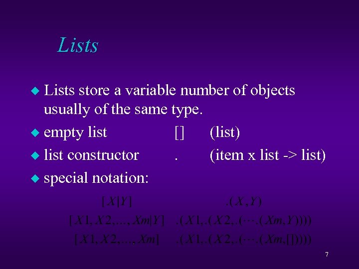Lists store a variable number of objects usually of the same type. u empty list [] (list) u list constructor. (item x list -> list) u special notation: u 7

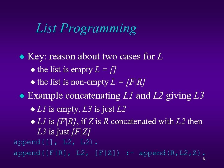List Programming u Key: reason about two cases for L u the list is empty L = [] u the list is non-empty L = [F|R] u Example concatenating L 1 and L 2 giving L 3 u L 1 is empty, L 3 is just L 2 u L 1 is [F|R], if Z is R concatenated with L 2 then L 3 is just [F|Z] append([], L 2). append([F|R], L 2, [F|Z]) : - append(R, L 2, Z). 8

Concatenation Examples append([], L 2). append([F|R], L 2, [F|Z]) : - append(R, L 2, Z). • concatenating lists append([1, 2], [3, 4], L) • has answer L = [1, 2, 3, 4] • breaking up lists append(X, Y, [1, 2]) • ans X=[]/Y=[1, 2], X=[1]/Y=[2], X=[1, 2]/Y=[] • BUT is a list equal to itself plus [1] • append(L, [1], L) runs forever! 9

Alldifferent Example We can program alldifferent using disequations alldifferent_neq([]). alldifferent_neq([Y|Ys]) : not_member(Y, Ys), alldifferent_neq(Ys). not_member(_, []). not_member(X, [Y|Ys]) : X != Y, not_member(X, Ys). The goal alldifferent_neq([A, B, C]) has one solution 10

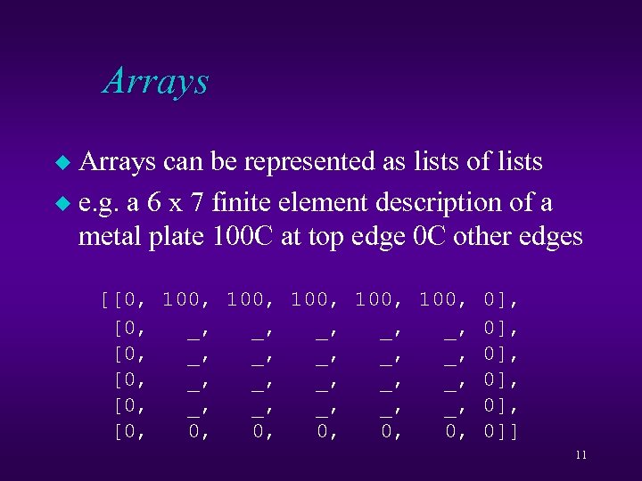Arrays can be represented as lists of lists u e. g. a 6 x 7 finite element description of a metal plate 100 C at top edge 0 C other edges u [[0, 100, 100, 0], [0, _, _, _, _, _, 0], [0, 0, 0, 0]] 11

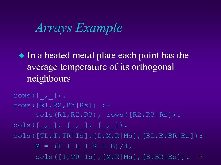Arrays Example u In a heated metal plate each point has the average temperature of its orthogonal neighbours rows([_, _]). rows([R 1, R 2, R 3|Rs]) : cols(R 1, R 2, R 3), rows([R 2, R 3|Rs]). cols([_, _], [_, _]). cols([TL, T, TR|Ts], [L, M, R|Ms], [BL, B, BR|Bs]): M = (T + L + R + B)/4, cols([T, TR|Ts], [M, R|Ms], [B, BR|Bs]). 12

Arrays Example u The goal rows(plate)constrains plate to [[0, 100, 100, 0], [0, 46. 6, 62. 5, 66. 4, 62. 5, 46. 6, 0], [0, 24. 0, 36. 9, 40. 8, 36. 9, 24. 0, 0], [0, 12. 4, 20. 3, 22. 9, 20. 3, 12. 4, 0], [0, 5. 3, 9. 0, 10. 2, 9. 0, 5. 3, 0], [0, 0, 0, 0]] 13

Association Lists A list of pairs is an association list u we can access the pair using only one half of the information u e. g. telephone book [p(peter, 5551616), p(kim, 5559282), p(nicole, 5559282)] u call this phonelist 14 u

List Membership member(X, [X|_]). member(X, [_|R]) : - member(X, R). X is a member of a list if it is the first element or it is a member of the remainder R We can use it to look up Kim’s phone number member(p(kim, N), phonelist) Unique answer: N = 5559282 15

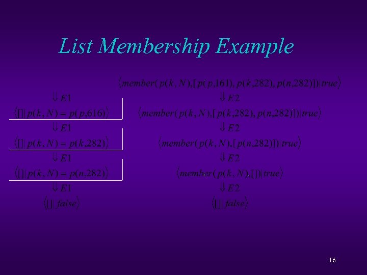List Membership Example 16

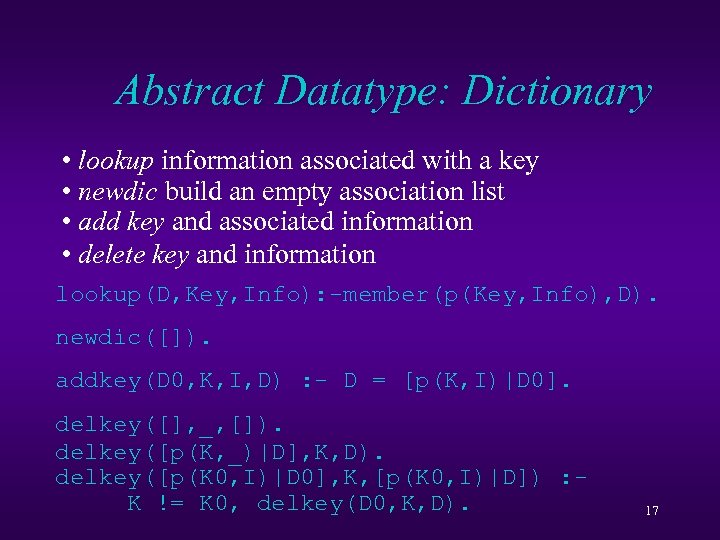Abstract Datatype: Dictionary • lookup information associated with a key • newdic build an empty association list • add key and associated information • delete key and information lookup(D, Key, Info): -member(p(Key, Info), D). newdic([]). addkey(D 0, K, I, D) : - D = [p(K, I)|D 0]. delkey([], _, []). delkey([p(K, _)|D], K, D). delkey([p(K 0, I)|D 0], K, [p(K 0, I)|D]) : K != K 0, delkey(D 0, K, D). 17

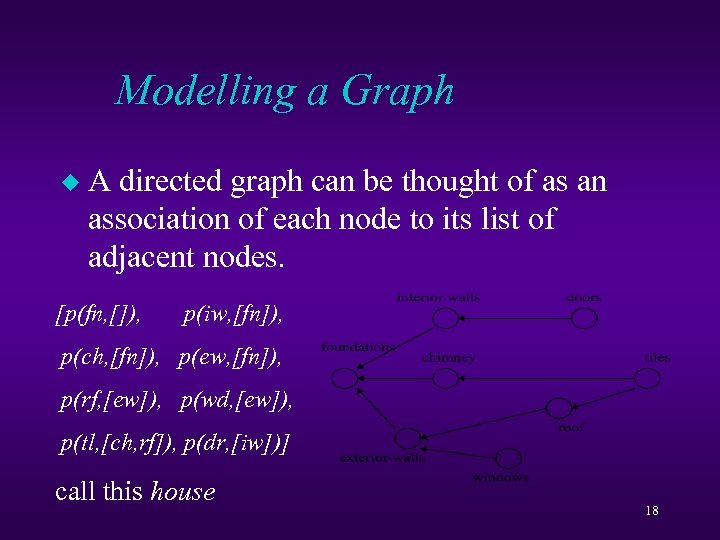Modelling a Graph u A directed graph can be thought of as an association of each node to its list of adjacent nodes. [p(fn, []), p(iw, [fn]), p(ch, [fn]), p(ew, [fn]), p(rf, [ew]), p(wd, [ew]), p(tl, [ch, rf]), p(dr, [iw])] call this house 18

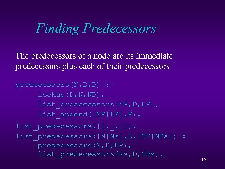Finding Predecessors The predecessors of a node are its immediate predecessors plus each of their predecessors(N, D, P) : lookup(D, N, NP), list_predecessors(NP, D, LP), list_append([NP|LP], P). list_predecessors([], _, []). list_predecessors([N|Ns], D, [NP|NPs]) : predecessors(N, D, NP), list_predecessors(Ns, D, NPs). 19

Finding Predecessors list_append([], []). list_append([L|Ls], All) : list_append(Ls, A), append(L, A, All). Appends a list of lists into one list. We can determine the predecessors of tiles (tl) using: predecessors(tl, house, Pre) The answer is Pre = [ch, rf, fn, ew, fn] Note repeated discovery of fn 20

Accumulation Programs building an answer sometimes can use the list answer calculated so far to improve the computation u Rather than one argument, the answer, use two arguments, the answer so far, and the final answer. u This is an accumulator pair u 21

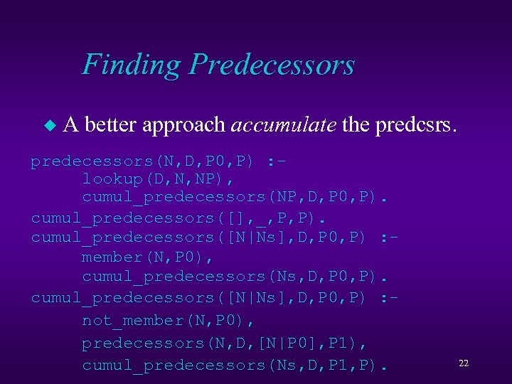Finding Predecessors u A better approach accumulate the predcsrs. predecessors(N, D, P 0, P) : lookup(D, N, NP), cumul_predecessors(NP, D, P 0, P). cumul_predecessors([], _, P, P). cumul_predecessors([N|Ns], D, P 0, P) : member(N, P 0), cumul_predecessors(Ns, D, P 0, P). cumul_predecessors([N|Ns], D, P 0, P) : not_member(N, P 0), predecessors(N, D, [N|P 0], P 1), cumul_predecessors(Ns, D, P 1, P). 22

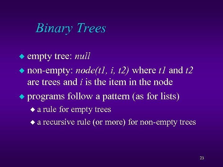Binary Trees empty tree: null u non-empty: node(t 1, i, t 2) where t 1 and t 2 are trees and i is the item in the node u programs follow a pattern (as for lists) u ua rule for empty trees u a recursive rule (or more) for non-empty trees 23

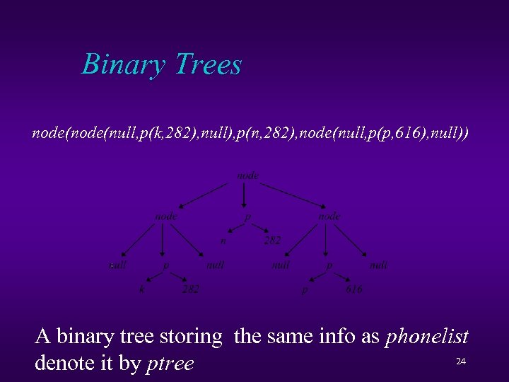Binary Trees node(null, p(k, 282), null), p(n, 282), node(null, p(p, 616), null)) A binary tree storing the same info as phonelist 24 denote it by ptree

Binary Trees traverse(null, []). traverse(node(T 1, I, T 2), L) : traverse(T 1, L 1), traverse(T 2, L 2), append(L 1, [I|L 2], L). Program to traverse a binary tree collecting items traverse(ptree, L) has unique answer L = [p(k, 282), p(n, 282), p(p, 616)] 25

Binary Search Tree binary search tree (BST): A binary tree with an order on the items such that for each node(t 1, i, t 2), each item in t 1 is less than i, and each item in t 2 is greater then i u previous example is a bst with right order u another implementation of a dictionary! u 26

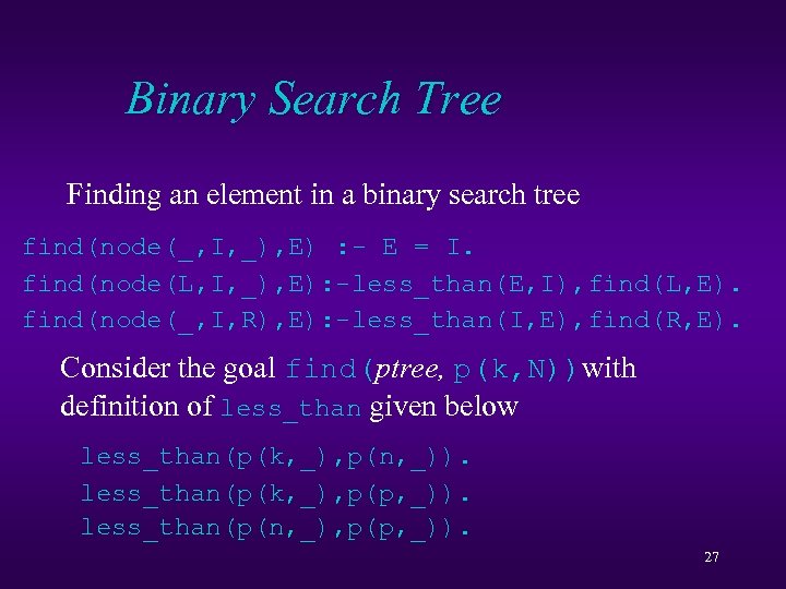Binary Search Tree Finding an element in a binary search tree find(node(_, I, _), E) : - E = I. find(node(L, I, _), E): -less_than(E, I), find(L, E). find(node(_, I, R), E): -less_than(I, E), find(R, E). Consider the goal find(ptree, p(k, N))with definition of less_than given below less_than(p(k, _), p(n, _)). less_than(p(k, _), p(p, _)). less_than(p(n, _), p(p, _)). 27

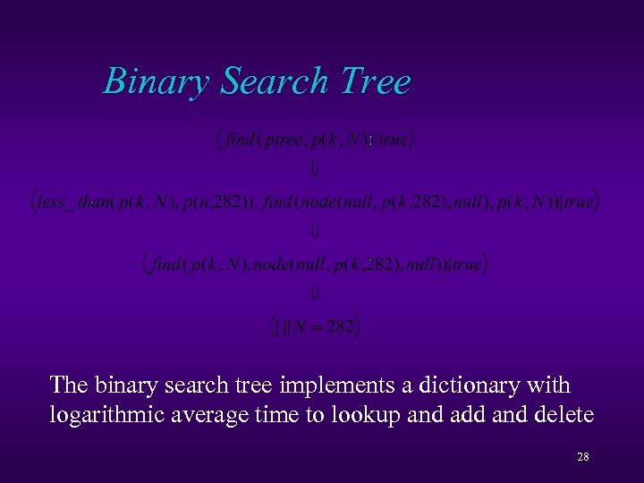Binary Search Tree The binary search tree implements a dictionary with logarithmic average time to lookup and add and delete 28

Hierarchical Modelling Many problems are hierarchical in nature u complex objects are made up of collections of simpler objects u modelling can reflect the hierarchy of the problem u 29

Hierarchical Modelling Ex. u steady-state RLC electrical circuits u sinusoidal voltages and currents are modelled by complex numbers: u individual circuit elements are modelled in terms of voltages and current: u circuits are modelled by combining circuit components 30

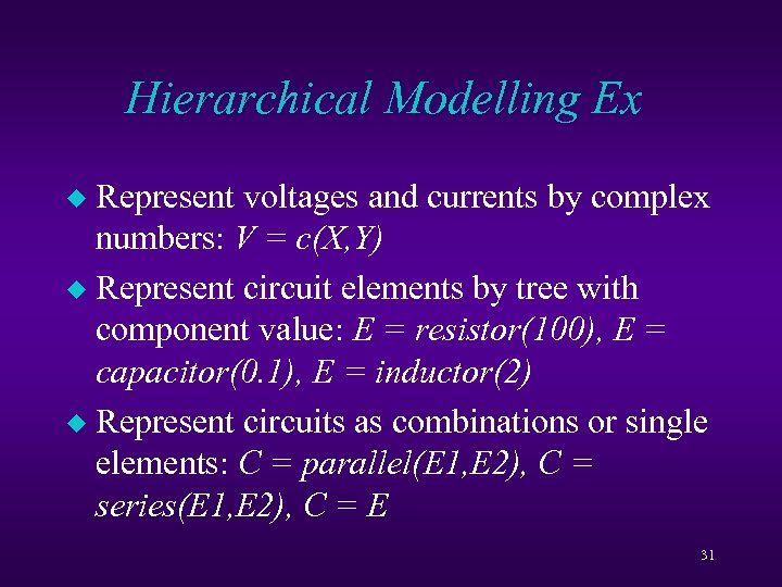Hierarchical Modelling Ex Represent voltages and currents by complex numbers: V = c(X, Y) u Represent circuit elements by tree with component value: E = resistor(100), E = capacitor(0. 1), E = inductor(2) u Represent circuits as combinations or single elements: C = parallel(E 1, E 2), C = series(E 1, E 2), C = E u 31

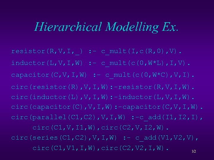Hierarchical Modelling Ex. resistor(R, V, I, _) : - c_mult(I, c(R, 0), V). inductor(L, V, I, W) : - c_mult(c(0, W*L), I, V). capacitor(C, V, I, W) : - c_mult(c(0, W*C), V, I). circ(resistor(R), V, I, W): -resistor(R, V, I, W). circ(inductor(L), V, I, W): -inductor(L, V, I, W). circ(capacitor(C), V, I, W): -capacitor(C, V, I, W). circ(parallel(C 1, C 2), V, I, W) : -c_add(I 1, I 2, I), circ(C 1, V, I 1, W), circ(C 2, V, I 2, W). circ(series(C 1, C 2), V, I, W) : - c_add(V 1, V 2, V), circ(C 1, V 1, I, W), circ(C 2, V 2, I, W). 32

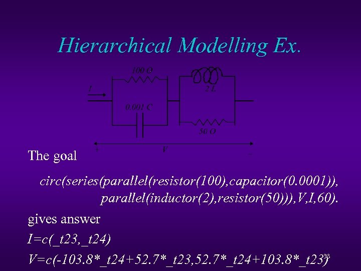Hierarchical Modelling Ex. The goal circ(series(parallel(resistor(100), capacitor(0. 0001)), parallel(inductor(2), resistor(50))), V, I, 60). gives answer I=c(_t 23, _t 24) 33 V=c(-103. 8*_t 24+52. 7*_t 23, 52. 7*_t 24+103. 8*_t 23)

Tree Layout Example u Drawing a good tree layout is difficult by hand. One approach is using constraints u Nodes at the same level are aligned horizontal u Different levels are spaced 10 apart u Minimum gap 10 between adjacent nodes on the same level u Parent node is above and midway between children u Width of the tree is minimized 34

Tree Layout Example u We can write a CLP program that given a tree finds a layout that satisfies these constraints ua association list to map a node to coordinates u predicates for building the constraints u predicate to calculate width u a minimization goal 35

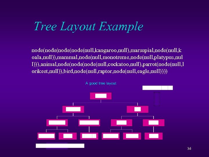Tree Layout Example node(node(null, kangaroo, null), marsupial, node(null, k oala, null)), mammal, node(null, monotreme, node(null, platypus, nul l))), animal, node(node(null, cockatoo, null), parrot(node(null, l orikeet, null)), bird, node(null, raptor, node(null, eagle, null)))) 36

Data Structures Summary u Tree constraints provide data structures u accessing and building in the same manner Records, lists and trees are straightforward u Programs reflect the form of the data struct. u Association lists are useful data structure for attaching information to objects u Hierarchical modelling u 37