e9e3043df3d177af2994eba954540c28.ppt
- Количество слайдов: 80
Chapter 6 The Normal Distribution © Mc. Graw-Hill, Bluman, 5 th ed. , Chapter 6 1
Chapter 6 Overview Introduction n 6 -1 Normal Distributions n 6 -2 Applications of the Normal Distribution n 6 -3 The Central Limit Theorem n 6 -4 The Normal Approximation to the Binomial Distribution Bluman, Chapter 6 2
Chapter 6 Objectives 1. Identify distributions as symmetric or skewed. 2. Identify the properties of a normal distribution. 3. Find the area under the standard normal distribution, given various z values. 4. Find probabilities for a normally distributed variable by transforming it into a standard normal variable. Bluman, Chapter 6 3
Chapter 6 Objectives 5. Find specific data values for given percentages, using the standard normal distribution. 6. Use the central limit theorem to solve problems involving sample means for large samples. 7. Use the normal approximation to compute probabilities for a binomial variable. Bluman, Chapter 6 4
6. 1 Normal Distributions n n Many continuous variables have distributions that are bell-shaped and are called approximately normally distributed variables The theoretical curve, called the bell curve or the Gaussian distribution, can be used to distribution study many variables that are not normally distributed but are approximately normal. Bluman, Chapter 6 5
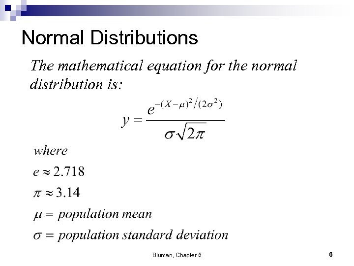
Normal Distributions The mathematical equation for the normal distribution is: Bluman, Chapter 6 6
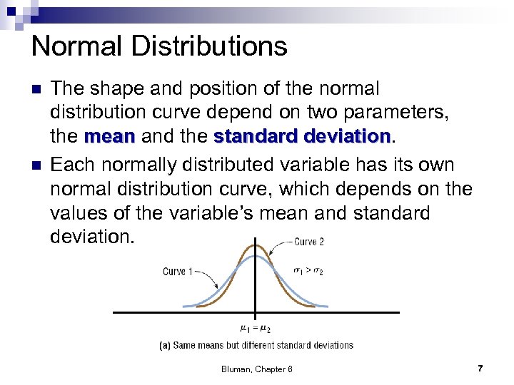
Normal Distributions n n The shape and position of the normal distribution curve depend on two parameters, the mean and the standard deviation Each normally distributed variable has its own normal distribution curve, which depends on the values of the variable’s mean and standard deviation. Bluman, Chapter 6 7
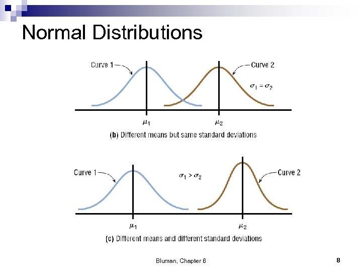
Normal Distributions Bluman, Chapter 6 8
Normal Distribution Properties n n The normal distribution curve is bell-shaped. The mean, median, and mode are equal and located at the center of the distribution. The normal distribution curve is unimodal (i. e. , it has only one mode). The curve is symmetrical about the mean, which is equivalent to saying that its shape is the same on both sides of a vertical line passing through the center. Bluman, Chapter 6 9
Normal Distribution Properties n n The curve is continuous—i. e. , there are no gaps or holes. For each value of X, here is a corresponding value of Y. The curve never touches the x axis. Theoretically, no matter how far in either direction the curve extends, it never meets the x axis—but it gets increasingly closer. Bluman, Chapter 6 10
Normal Distribution Properties n n The total area under the normal distribution curve is equal to 1. 00 or 100%. The area under the normal curve that lies within ¨ one standard deviation of the mean is approximately 0. 68 (68%). ¨ two standard deviations of the mean is approximately 0. 95 (95%). ¨ three standard deviations of the mean is approximately 0. 997 ( 99. 7%). Bluman, Chapter 6 11
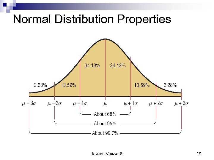
Normal Distribution Properties Bluman, Chapter 6 12
Standard Normal Distribution n n Since each normally distributed variable has its own mean and standard deviation, the shape and location of these curves will vary. In practical applications, one would have to have a table of areas under the curve for each variable. To simplify this, statisticians use the standard normal distribution. The standard normal distribution is a normal distribution with a mean of 0 and a standard deviation of 1. Bluman, Chapter 6 13
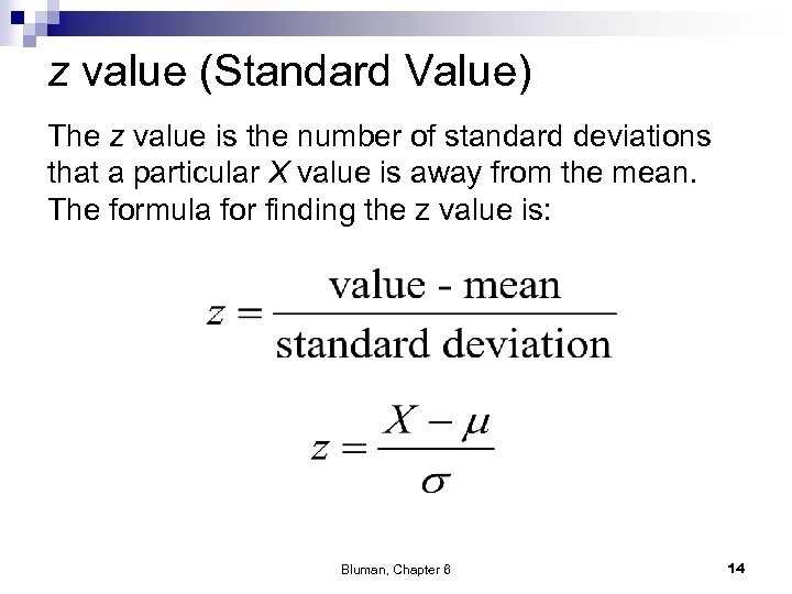
z value (Standard Value) The z value is the number of standard deviations that a particular X value is away from the mean. The formula for finding the z value is: Bluman, Chapter 6 14
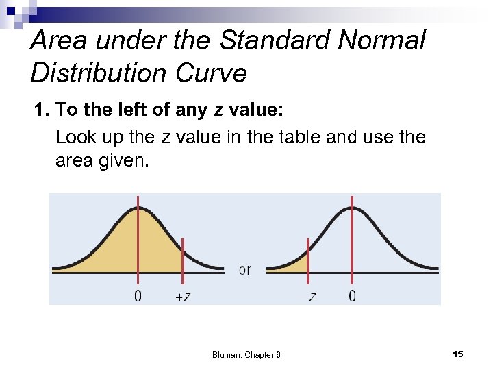
Area under the Standard Normal Distribution Curve 1. To the left of any z value: Look up the z value in the table and use the area given. Bluman, Chapter 6 15
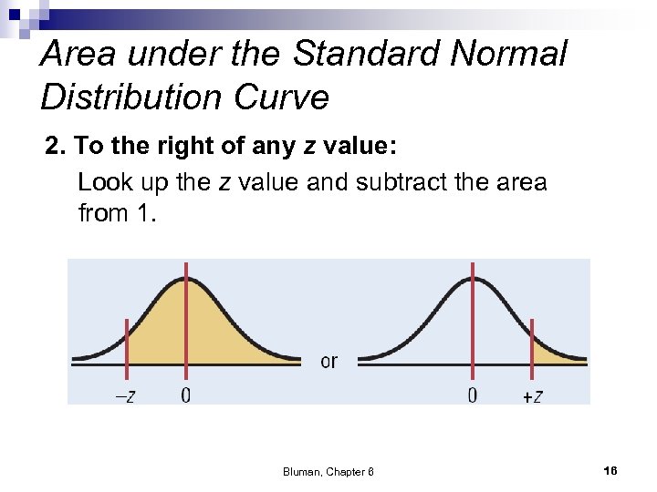
Area under the Standard Normal Distribution Curve 2. To the right of any z value: Look up the z value and subtract the area from 1. Bluman, Chapter 6 16
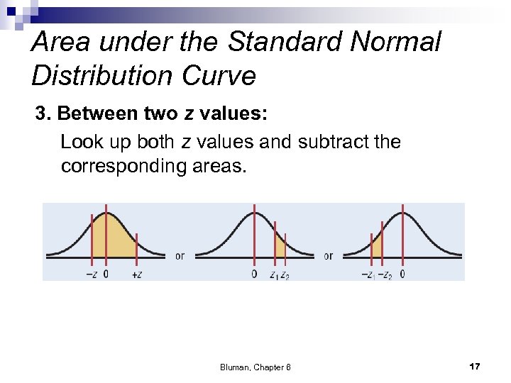
Area under the Standard Normal Distribution Curve 3. Between two z values: Look up both z values and subtract the corresponding areas. Bluman, Chapter 6 17

Chapter 6 Normal Distributions Section 6 -1 Example 6 -1 Page #306 Bluman, Chapter 6 18
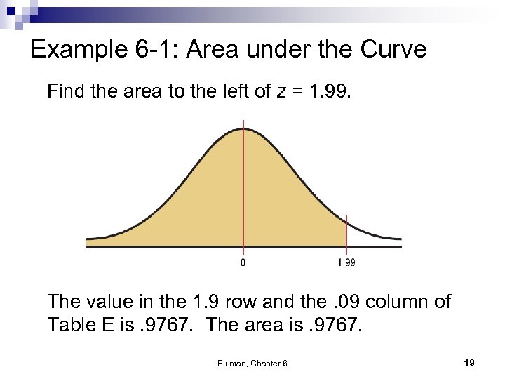
Example 6 -1: Area under the Curve Find the area to the left of z = 1. 99. The value in the 1. 9 row and the. 09 column of Table E is. 9767. The area is. 9767. Bluman, Chapter 6 19
Chapter 6 Normal Distributions Section 6 -1 Example 6 -2 Page #306 Bluman, Chapter 6 20
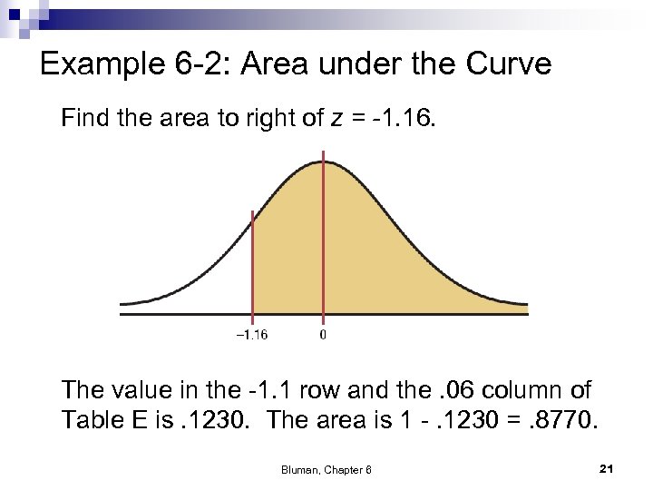
Example 6 -2: Area under the Curve Find the area to right of z = -1. 16. The value in the -1. 1 row and the. 06 column of Table E is. 1230. The area is 1 -. 1230 =. 8770. Bluman, Chapter 6 21

Chapter 6 Normal Distributions Section 6 -1 Example 6 -3 Page #307 Bluman, Chapter 6 22
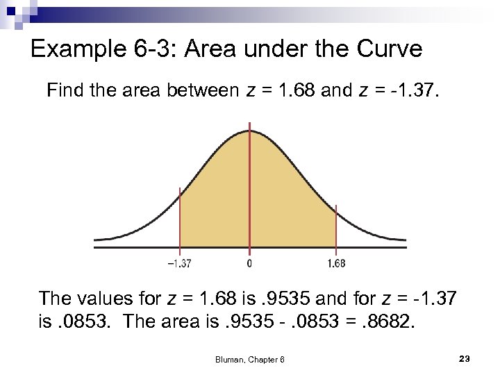
Example 6 -3: Area under the Curve Find the area between z = 1. 68 and z = -1. 37. The values for z = 1. 68 is. 9535 and for z = -1. 37 is. 0853. The area is. 9535 -. 0853 =. 8682. Bluman, Chapter 6 23

Chapter 6 Normal Distributions Section 6 -1 Example 6 -4 Page #308 Bluman, Chapter 6 24
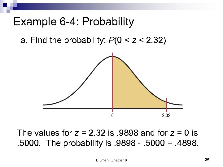
Example 6 -4: Probability a. Find the probability: P(0 < z < 2. 32) The values for z = 2. 32 is. 9898 and for z = 0 is. 5000. The probability is. 9898 -. 5000 =. 4898. Bluman, Chapter 6 25
Chapter 6 Normal Distributions Section 6 -1 Example 6 -5 Page #309 Bluman, Chapter 6 26
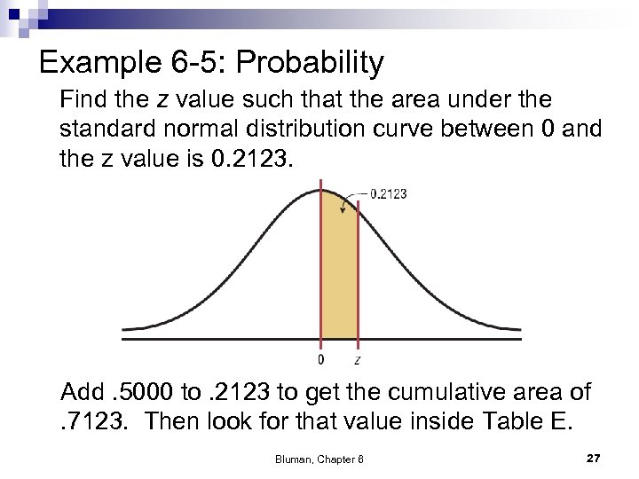
Example 6 -5: Probability Find the z value such that the area under the standard normal distribution curve between 0 and the z value is 0. 2123. Add. 5000 to. 2123 to get the cumulative area of. 7123. Then look for that value inside Table E. Bluman, Chapter 6 27
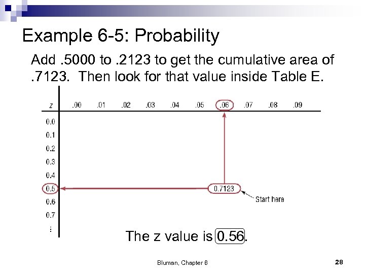
Example 6 -5: Probability Add. 5000 to. 2123 to get the cumulative area of. 7123. Then look for that value inside Table E. The z value is 0. 56. Bluman, Chapter 6 28
6. 2 Applications of the Normal Distributions n n The standard normal distribution curve can be used to solve a wide variety of practical problems. The only requirement is that the variable be normally or approximately normally distributed. For all the problems presented in this chapter, you can assume that the variable is normally or approximately normally distributed. Bluman, Chapter 6 29
Applications of the Normal Distributions n n To solve problems by using the standard normal distribution, transform the original variable to a standard normal distribution variable by using the z value formula. This formula transforms the values of the variable into standard units or z values. Once the variable is transformed, then the Procedure Table and Table E in Appendix C can be used to solve problems. Bluman, Chapter 6 30
Chapter 6 Normal Distributions Section 6 -2 Example 6 -6 Page #317 Bluman, Chapter 6 31
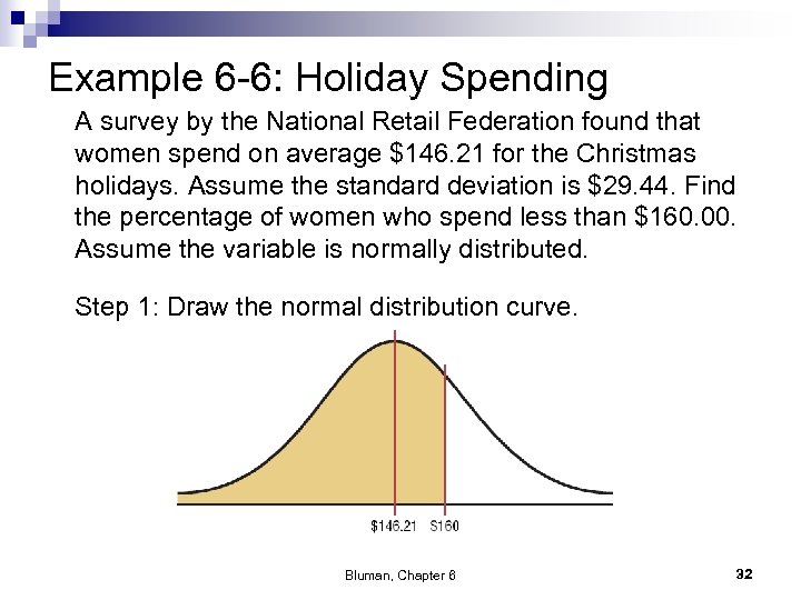
Example 6 -6: Holiday Spending A survey by the National Retail Federation found that women spend on average $146. 21 for the Christmas holidays. Assume the standard deviation is $29. 44. Find the percentage of women who spend less than $160. 00. Assume the variable is normally distributed. Step 1: Draw the normal distribution curve. Bluman, Chapter 6 32
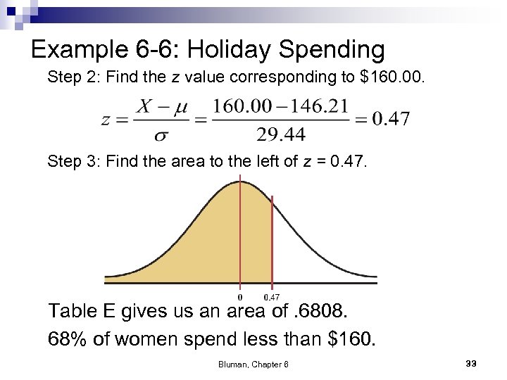
Example 6 -6: Holiday Spending Step 2: Find the z value corresponding to $160. 00. Step 3: Find the area to the left of z = 0. 47. Table E gives us an area of. 6808. 68% of women spend less than $160. Bluman, Chapter 6 33

Chapter 6 Normal Distributions Section 6 -2 Example 6 -7 a Page #317 Bluman, Chapter 6 34
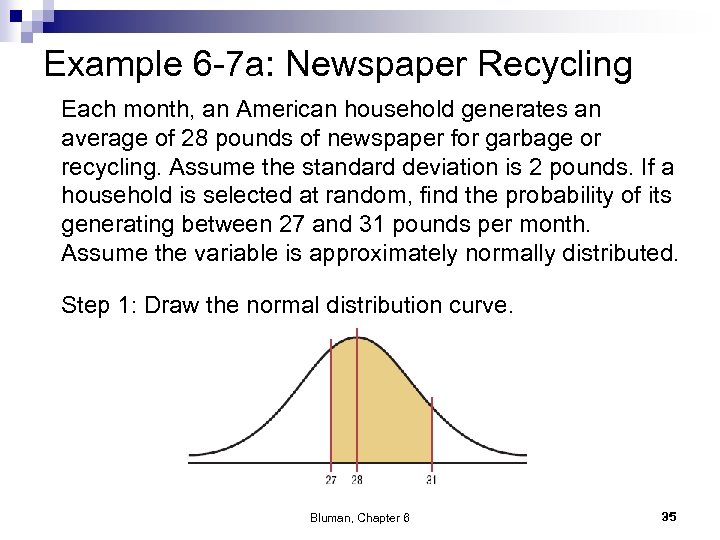
Example 6 -7 a: Newspaper Recycling Each month, an American household generates an average of 28 pounds of newspaper for garbage or recycling. Assume the standard deviation is 2 pounds. If a household is selected at random, find the probability of its generating between 27 and 31 pounds per month. Assume the variable is approximately normally distributed. Step 1: Draw the normal distribution curve. Bluman, Chapter 6 35
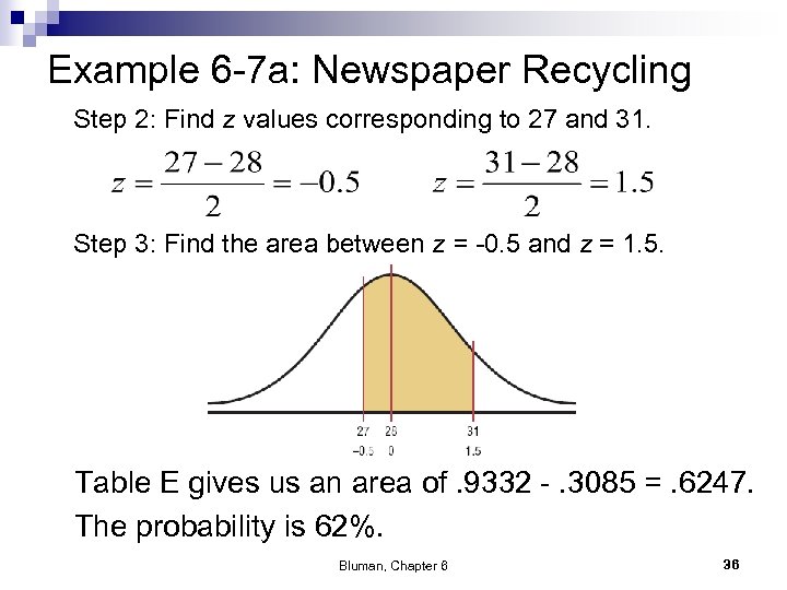
Example 6 -7 a: Newspaper Recycling Step 2: Find z values corresponding to 27 and 31. Step 3: Find the area between z = -0. 5 and z = 1. 5. Table E gives us an area of. 9332 -. 3085 =. 6247. The probability is 62%. Bluman, Chapter 6 36

Chapter 6 Normal Distributions Section 6 -2 Example 6 -8 Page #319 Bluman, Chapter 6 37
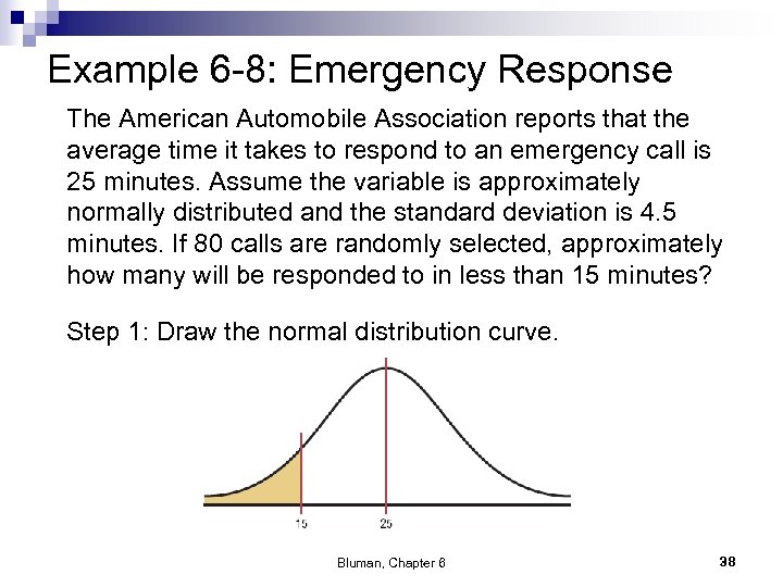
Example 6 -8: Emergency Response The American Automobile Association reports that the average time it takes to respond to an emergency call is 25 minutes. Assume the variable is approximately normally distributed and the standard deviation is 4. 5 minutes. If 80 calls are randomly selected, approximately how many will be responded to in less than 15 minutes? Step 1: Draw the normal distribution curve. Bluman, Chapter 6 38
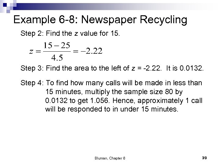
Example 6 -8: Newspaper Recycling Step 2: Find the z value for 15. Step 3: Find the area to the left of z = -2. 22. It is 0. 0132. Step 4: To find how many calls will be made in less than 15 minutes, multiply the sample size 80 by 0. 0132 to get 1. 056. Hence, approximately 1 call will be responded to in under 15 minutes. Bluman, Chapter 6 39

Chapter 6 Normal Distributions Section 6 -2 Example 6 -9 Page #320 Bluman, Chapter 6 40
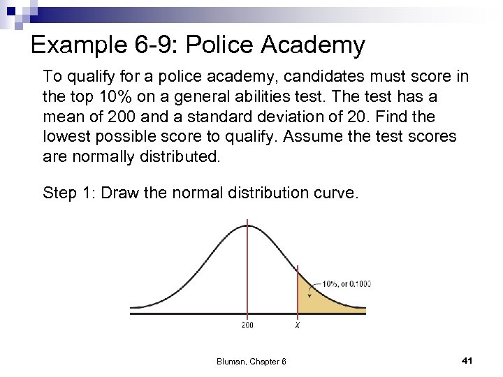
Example 6 -9: Police Academy To qualify for a police academy, candidates must score in the top 10% on a general abilities test. The test has a mean of 200 and a standard deviation of 20. Find the lowest possible score to qualify. Assume the test scores are normally distributed. Step 1: Draw the normal distribution curve. Bluman, Chapter 6 41
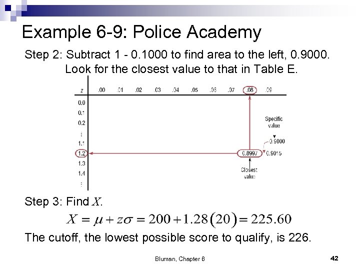
Example 6 -9: Police Academy Step 2: Subtract 1 - 0. 1000 to find area to the left, 0. 9000. Look for the closest value to that in Table E. Step 3: Find X. The cutoff, the lowest possible score to qualify, is 226. Bluman, Chapter 6 42

Chapter 6 Normal Distributions Section 6 -2 Example 6 -10 Page #321 Bluman, Chapter 6 43
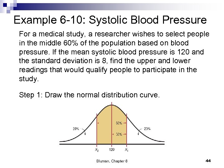
Example 6 -10: Systolic Blood Pressure For a medical study, a researcher wishes to select people in the middle 60% of the population based on blood pressure. If the mean systolic blood pressure is 120 and the standard deviation is 8, find the upper and lower readings that would qualify people to participate in the study. Step 1: Draw the normal distribution curve. Bluman, Chapter 6 44
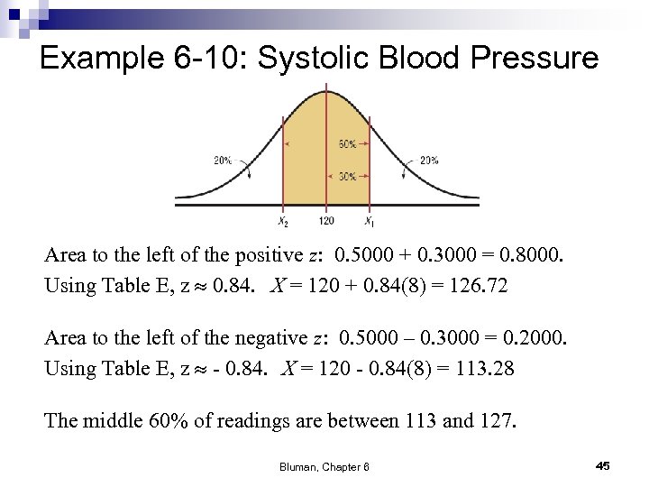
Example 6 -10: Systolic Blood Pressure Area to the left of the positive z: 0. 5000 + 0. 3000 = 0. 8000. Using Table E, z 0. 84. X = 120 + 0. 84(8) = 126. 72 Area to the left of the negative z: 0. 5000 – 0. 3000 = 0. 2000. Using Table E, z - 0. 84. X = 120 - 0. 84(8) = 113. 28 The middle 60% of readings are between 113 and 127. Bluman, Chapter 6 45
Normal Distributions n n A normally shaped or bell-shaped distribution is only one of many shapes that a distribution can assume; however, it is very important since many statistical methods require that the distribution of values (shown in subsequent chapters) be normally or approximately normally shaped. There a number of ways statisticians check for normality. We will focus on three of them. Bluman, Chapter 6 46
Checking for Normality Histogram n Pearson’s Index PI of Skewness n Outliers n Other Tests n ¨ Normal Quantile Plot ¨ Chi-Square Goodness-of-Fit Test ¨ Kolmogorov-Smikirov Test ¨ Lilliefors Test Bluman, Chapter 6 47

Chapter 6 Normal Distributions Section 6 -2 Example 6 -11 Page #322 Bluman, Chapter 6 48
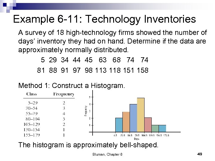
Example 6 -11: Technology Inventories A survey of 18 high-technology firms showed the number of days’ inventory they had on hand. Determine if the data are approximately normally distributed. 5 29 34 44 45 63 68 74 74 81 88 91 97 98 113 118 151 158 Method 1: Construct a Histogram. The histogram is approximately bell-shaped. Bluman, Chapter 6 49
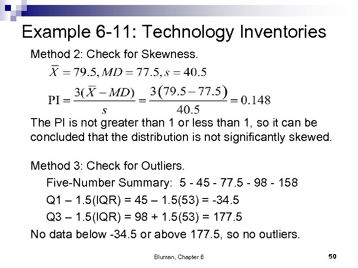
Example 6 -11: Technology Inventories Method 2: Check for Skewness. The PI is not greater than 1 or less than 1, so it can be concluded that the distribution is not significantly skewed. Method 3: Check for Outliers. Five-Number Summary: 5 - 45 - 77. 5 - 98 - 158 Q 1 – 1. 5(IQR) = 45 – 1. 5(53) = -34. 5 Q 3 – 1. 5(IQR) = 98 + 1. 5(53) = 177. 5 No data below -34. 5 or above 177. 5, so no outliers. Bluman, Chapter 6 50
Example 6 -11: Technology Inventories A survey of 18 high-technology firms showed the number of days’ inventory they had on hand. Determine if the data are approximately normally distributed. 5 29 34 44 45 63 68 74 74 81 88 91 97 98 113 118 151 158 Conclusion: n The histogram is approximately bell-shaped. n The data are not significantly skewed. n There are no outliers. Thus, it can be concluded that the distribution is approximately normally distributed. Bluman, Chapter 6 51
6. 3 The Central Limit Theorem In addition to knowing how individual data values vary about the mean for a population, statisticians are interested in knowing how the means of samples of the same size taken from the same population vary about the population mean. Bluman, Chapter 6 52
Distribution of Sample Means n n A sampling distribution of sample means is a distribution obtained by using the means computed from random samples of a specific size taken from a population. Sampling error is the difference between the sample measure and the corresponding population measure due to the fact that the sample is not a perfect representation of the population. Bluman, Chapter 6 53
Properties of the Distribution of Sample Means n n The mean of the sample means will be the same as the population mean. The standard deviation of the sample means will be smaller than the standard deviation of the population, and will be equal to the population standard deviation divided by the square root of the sample size. Bluman, Chapter 6 54
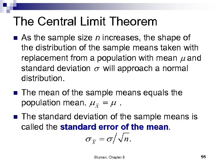
The Central Limit Theorem n As the sample size n increases, the shape of the distribution of the sample means taken with replacement from a population with mean and standard deviation will approach a normal distribution. n The mean of the sample means equals the population mean. . n The standard deviation of the sample means is called the standard error of the mean Bluman, Chapter 6 55
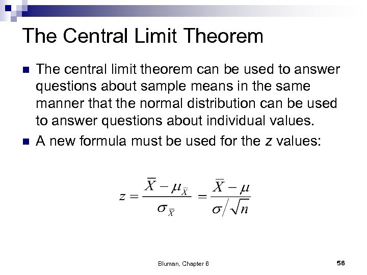
The Central Limit Theorem n n The central limit theorem can be used to answer questions about sample means in the same manner that the normal distribution can be used to answer questions about individual values. A new formula must be used for the z values: Bluman, Chapter 6 56

Chapter 6 Normal Distributions Section 6 -3 Example 6 -13 Page #334 Bluman, Chapter 6 57
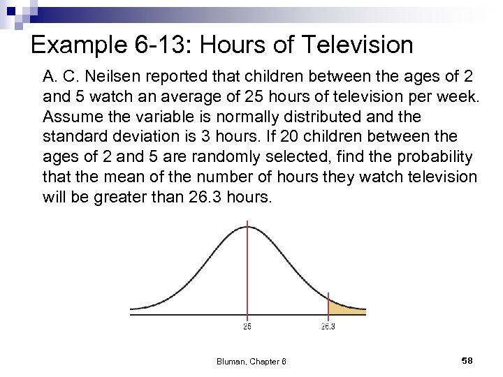
Example 6 -13: Hours of Television A. C. Neilsen reported that children between the ages of 2 and 5 watch an average of 25 hours of television per week. Assume the variable is normally distributed and the standard deviation is 3 hours. If 20 children between the ages of 2 and 5 are randomly selected, find the probability that the mean of the number of hours they watch television will be greater than 26. 3 hours. Bluman, Chapter 6 58
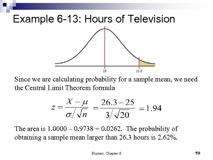
Example 6 -13: Hours of Television Since we are calculating probability for a sample mean, we need the Central Limit Theorem formula The area is 1. 0000 – 0. 9738 = 0. 0262. The probability of obtaining a sample mean larger than 26. 3 hours is 2. 62%. Bluman, Chapter 6 59

Chapter 6 Normal Distributions Section 6 -3 Example 6 -14 Page #335 Bluman, Chapter 6 60
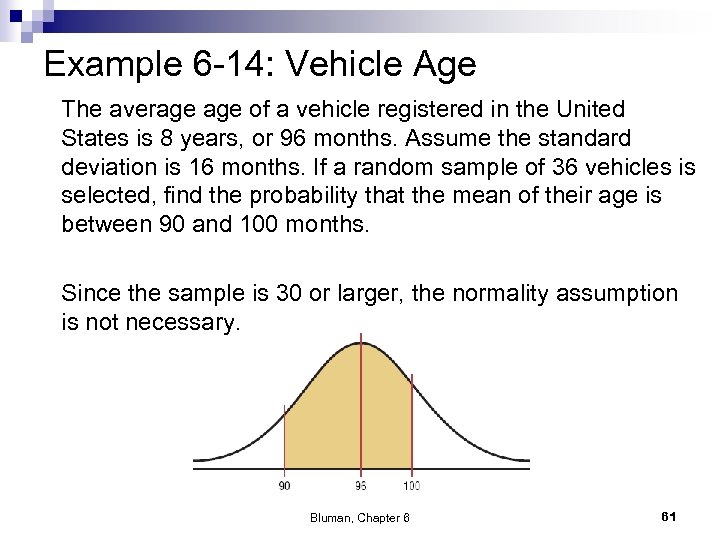
Example 6 -14: Vehicle Age The average of a vehicle registered in the United States is 8 years, or 96 months. Assume the standard deviation is 16 months. If a random sample of 36 vehicles is selected, find the probability that the mean of their age is between 90 and 100 months. Since the sample is 30 or larger, the normality assumption is not necessary. Bluman, Chapter 6 61
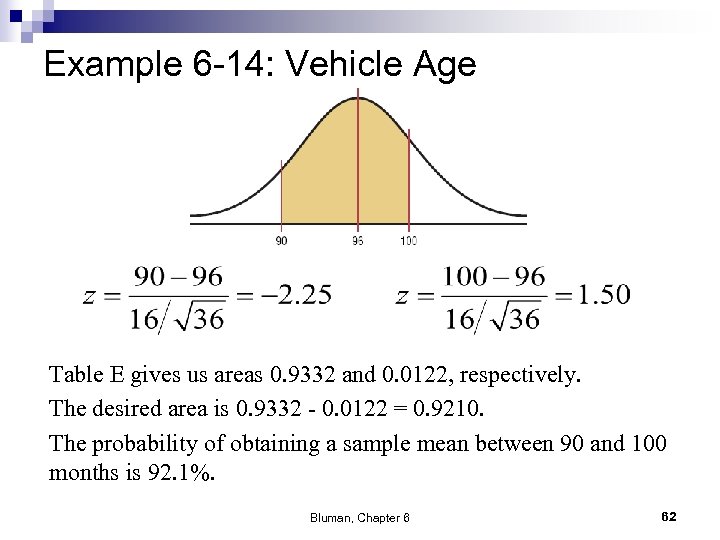
Example 6 -14: Vehicle Age Table E gives us areas 0. 9332 and 0. 0122, respectively. The desired area is 0. 9332 - 0. 0122 = 0. 9210. The probability of obtaining a sample mean between 90 and 100 months is 92. 1%. Bluman, Chapter 6 62
Chapter 6 Normal Distributions Section 6 -3 Example 6 -15 Page #336 Bluman, Chapter 6 63
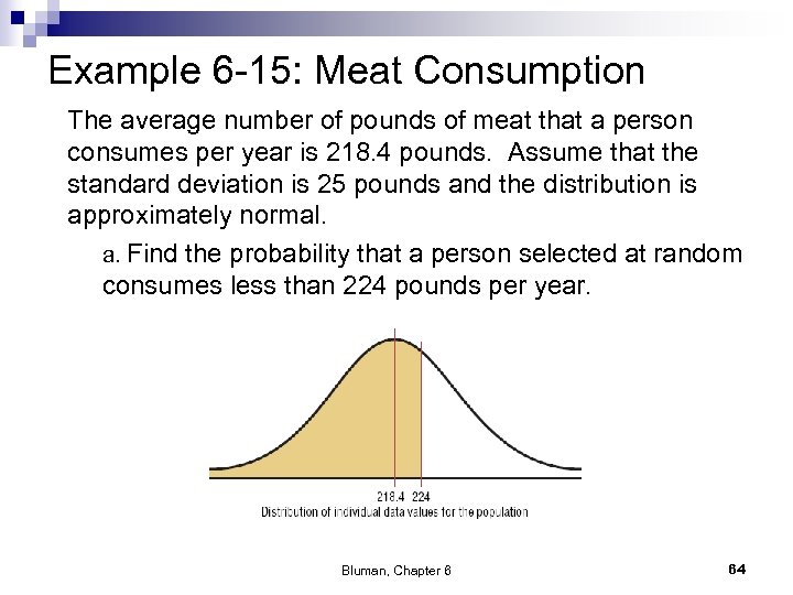
Example 6 -15: Meat Consumption The average number of pounds of meat that a person consumes per year is 218. 4 pounds. Assume that the standard deviation is 25 pounds and the distribution is approximately normal. a. Find the probability that a person selected at random consumes less than 224 pounds per year. Bluman, Chapter 6 64
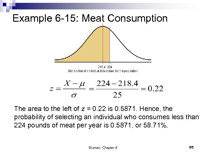
Example 6 -15: Meat Consumption The area to the left of z = 0. 22 is 0. 5871. Hence, the probability of selecting an individual who consumes less than 224 pounds of meat per year is 0. 5871, or 58. 71%. Bluman, Chapter 6 65
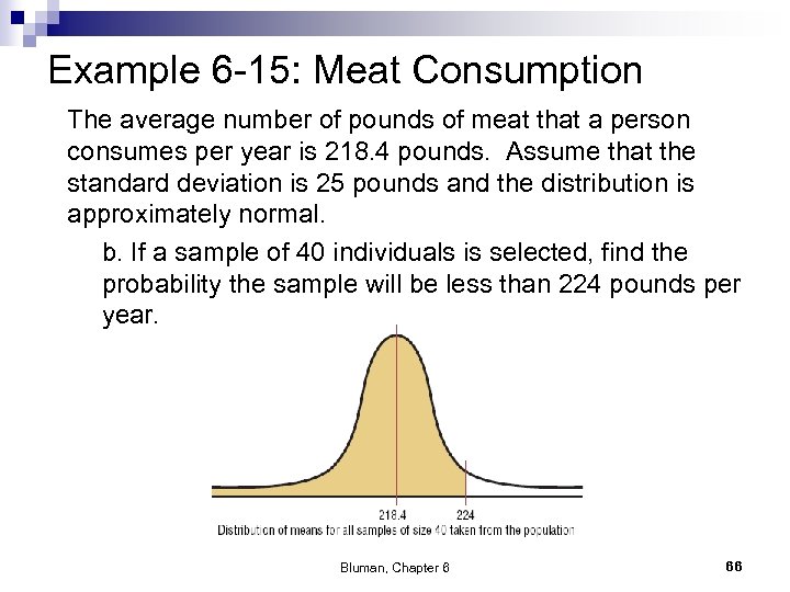
Example 6 -15: Meat Consumption The average number of pounds of meat that a person consumes per year is 218. 4 pounds. Assume that the standard deviation is 25 pounds and the distribution is approximately normal. b. If a sample of 40 individuals is selected, find the probability the sample will be less than 224 pounds per year. Bluman, Chapter 6 66
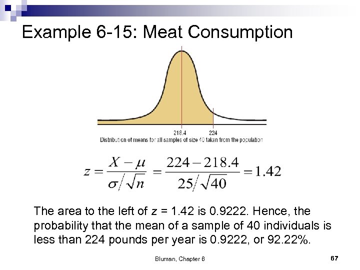
Example 6 -15: Meat Consumption The area to the left of z = 1. 42 is 0. 9222. Hence, the probability that the mean of a sample of 40 individuals is less than 224 pounds per year is 0. 9222, or 92. 22%. Bluman, Chapter 6 67
Finite Population Correction Factor n n The formula for standard error of the mean is accurate when the samples are drawn with replacement or are drawn without replacement from a very large or infinite population. A correction factor is necessary for computing the standard error of the mean for samples drawn without replacement from a finite population. Bluman, Chapter 6 68
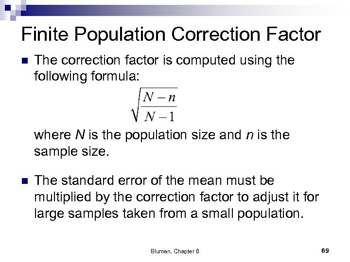
Finite Population Correction Factor n The correction factor is computed using the following formula: where N is the population size and n is the sample size. n The standard error of the mean must be multiplied by the correction factor to adjust it for large samples taken from a small population. Bluman, Chapter 6 69
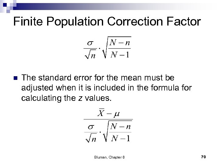
Finite Population Correction Factor n The standard error for the mean must be adjusted when it is included in the formula for calculating the z values. Bluman, Chapter 6 70
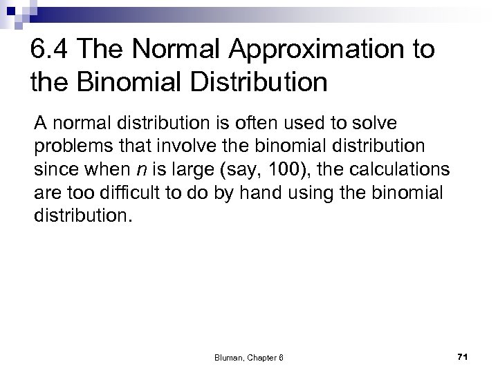
6. 4 The Normal Approximation to the Binomial Distribution A normal distribution is often used to solve problems that involve the binomial distribution since when n is large (say, 100), the calculations are too difficult to do by hand using the binomial distribution. Bluman, Chapter 6 71
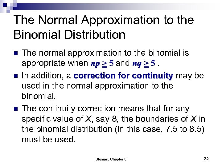
The Normal Approximation to the Binomial Distribution n The normal approximation to the binomial is appropriate when np > 5 and nq > 5. In addition, a correction for continuity may be used in the normal approximation to the binomial. The continuity correction means that for any specific value of X, say 8, the boundaries of X in the binomial distribution (in this case, 7. 5 to 8. 5) must be used. Bluman, Chapter 6 72
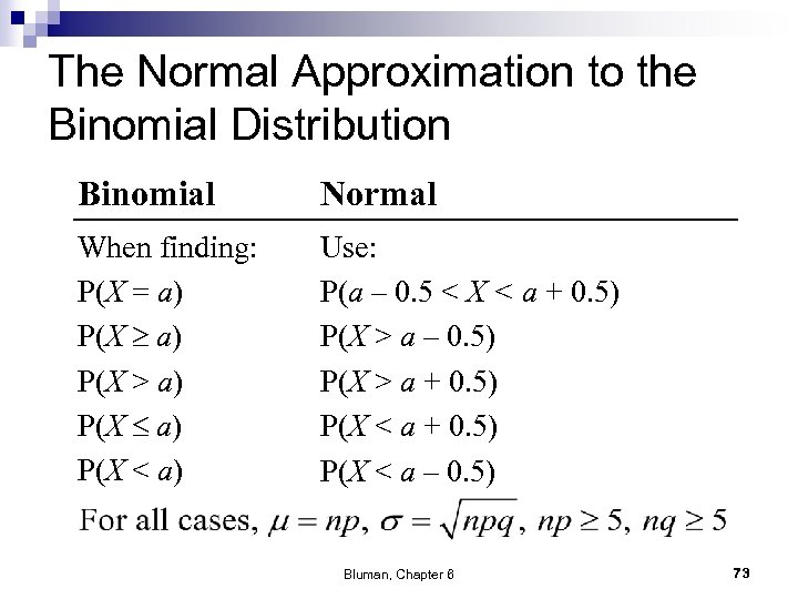
The Normal Approximation to the Binomial Distribution Binomial Normal When finding: P(X = a) P(X > a) P(X < a) Use: P(a – 0. 5 < X < a + 0. 5) P(X > a – 0. 5) P(X > a + 0. 5) P(X < a – 0. 5) Bluman, Chapter 6 73
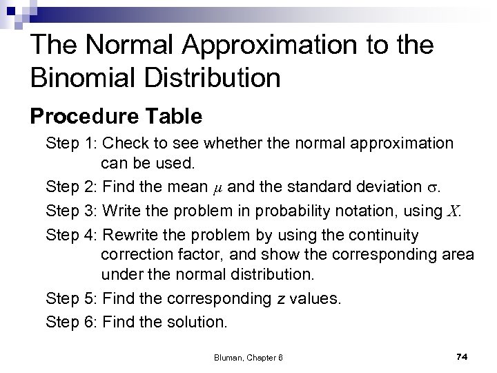
The Normal Approximation to the Binomial Distribution Procedure Table Step 1: Check to see whether the normal approximation can be used. Step 2: Find the mean µ and the standard deviation . Step 3: Write the problem in probability notation, using X. Step 4: Rewrite the problem by using the continuity correction factor, and show the corresponding area under the normal distribution. Step 5: Find the corresponding z values. Step 6: Find the solution. Bluman, Chapter 6 74

Chapter 6 Normal Distributions Section 6 -4 Example 6 -16 Page #343 Bluman, Chapter 6 75
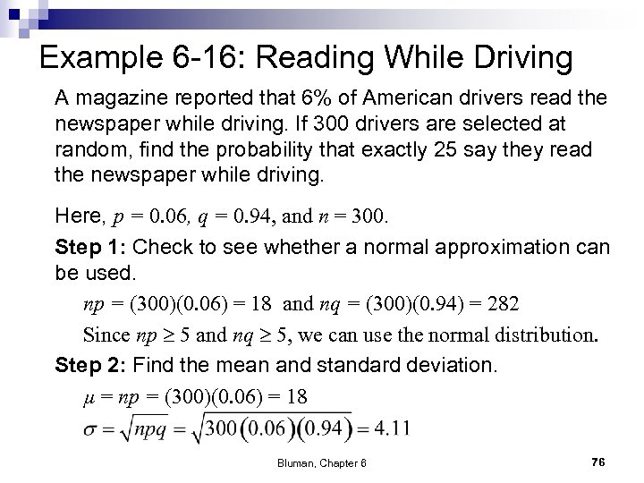
Example 6 -16: Reading While Driving A magazine reported that 6% of American drivers read the newspaper while driving. If 300 drivers are selected at random, find the probability that exactly 25 say they read the newspaper while driving. Here, p = 0. 06, q = 0. 94, and n = 300. Step 1: Check to see whether a normal approximation can be used. np = (300)(0. 06) = 18 and nq = (300)(0. 94) = 282 Since np 5 and nq 5, we can use the normal distribution. Step 2: Find the mean and standard deviation. µ = np = (300)(0. 06) = 18 Bluman, Chapter 6 76
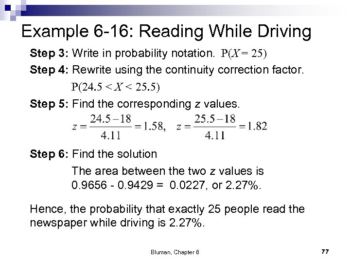
Example 6 -16: Reading While Driving Step 3: Write in probability notation. P(X = 25) Step 4: Rewrite using the continuity correction factor. P(24. 5 < X < 25. 5) Step 5: Find the corresponding z values. Step 6: Find the solution The area between the two z values is 0. 9656 - 0. 9429 = 0. 0227, or 2. 27%. Hence, the probability that exactly 25 people read the newspaper while driving is 2. 27%. Bluman, Chapter 6 77

Chapter 6 Normal Distributions Section 6 -4 Example 6 -17 Page #343 Bluman, Chapter 6 78
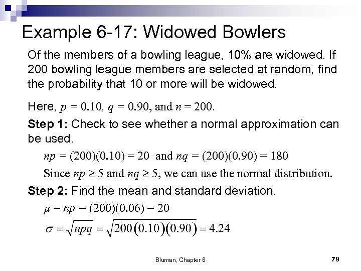
Example 6 -17: Widowed Bowlers Of the members of a bowling league, 10% are widowed. If 200 bowling league members are selected at random, find the probability that 10 or more will be widowed. Here, p = 0. 10, q = 0. 90, and n = 200. Step 1: Check to see whether a normal approximation can be used. np = (200)(0. 10) = 20 and nq = (200)(0. 90) = 180 Since np 5 and nq 5, we can use the normal distribution. Step 2: Find the mean and standard deviation. µ = np = (200)(0. 06) = 20 Bluman, Chapter 6 79
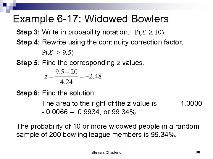
Example 6 -17: Widowed Bowlers Step 3: Write in probability notation. P(X 10) Step 4: Rewrite using the continuity correction factor. P(X > 9. 5) Step 5: Find the corresponding z values. Step 6: Find the solution The area to the right of the z value is - 0. 0066 = 0. 9934, or 99. 34%. 1. 0000 The probability of 10 or more widowed people in a random sample of 200 bowling league members is 99. 34%. Bluman, Chapter 6 80
e9e3043df3d177af2994eba954540c28.ppt