Chapter 6 Spatial Joins Outline

Chapter 6 Spatial Joins

Outline • • • Spatial joins Cardinality Types of spatial joins Feature geometry and distance joins Coordinate systems and distance joins

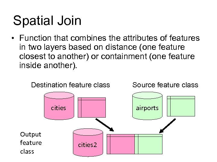Spatial Join • Function that combines the attributes of features in two layers based on distance (one feature closest to another) or containment (one feature inside another). Destination feature class cities Output feature class Source feature class airports cities 2

Cardinality • Relationship between records in two tables : – Simple joins • One-to-one or many-to-one cardinality – Summarized joins • One-to-many or many-to-many

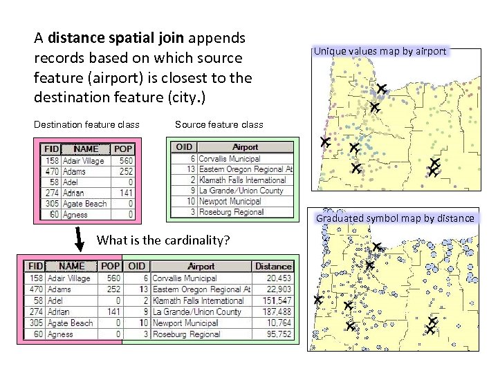A distance spatial join appends records based on which source feature (airport) is closest to the destination feature (city. ) Destination feature class Unique values map by airport Source feature class Graduated symbol map by distance What is the cardinality?

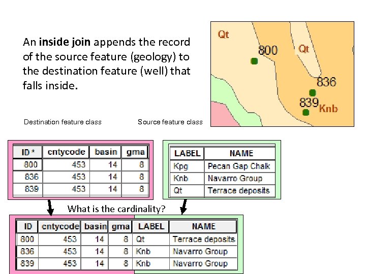An inside join appends the record of the source feature (geology) to the destination feature (well) that falls inside. Destination feature class Source feature class What is the cardinality?

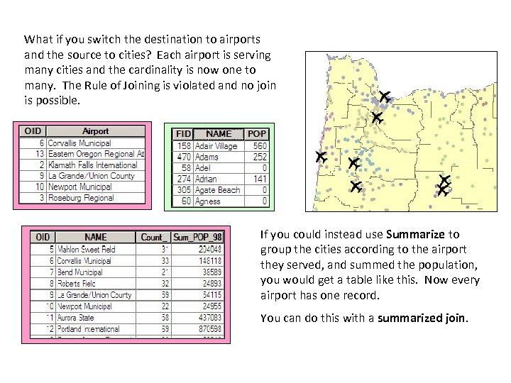What if you switch the destination to airports and the source to cities? Each airport is serving many cities and the cardinality is now one to many. The Rule of Joining is violated and no join is possible. If you could instead use Summarize to group the cities according to the airport they served, and summed the population, you would get a table like this. Now every airport has one record. You can do this with a summarized join.

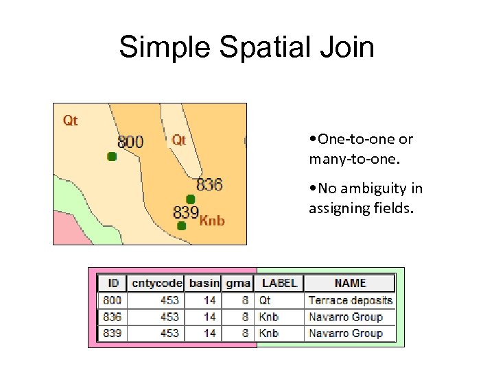Simple Spatial Join • One-to-one or many-to-one. • No ambiguity in assigning fields.

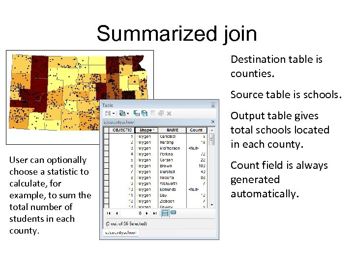Summarized join Destination table is counties. Source table is schools. Output table gives total schools located in each county. User can optionally choose a statistic to calculate, for example, to sum the total number of students in each county. Count field is always generated automatically.

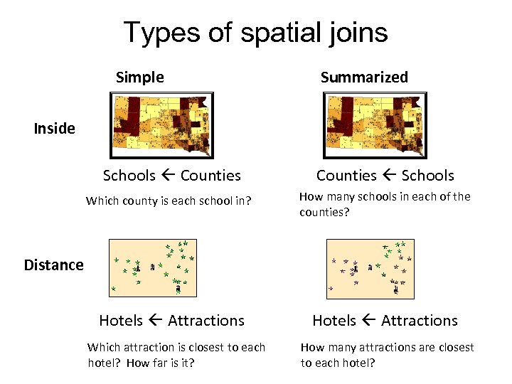Types of spatial joins Simple Summarized Inside Schools Counties Schools Which county is each school in? How many schools in each of the counties? Hotels Attractions Distance Which attraction is closest to each hotel? How far is it? How many attractions are closest to each hotel?

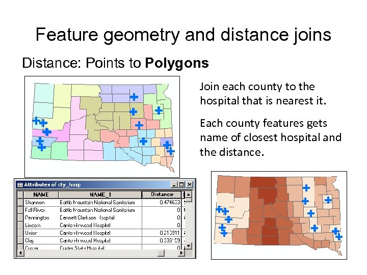Feature geometry and distance joins Distance: Points to Polygons Join each county to the hospital that is nearest it. Each county features gets name of closest hospital and the distance.

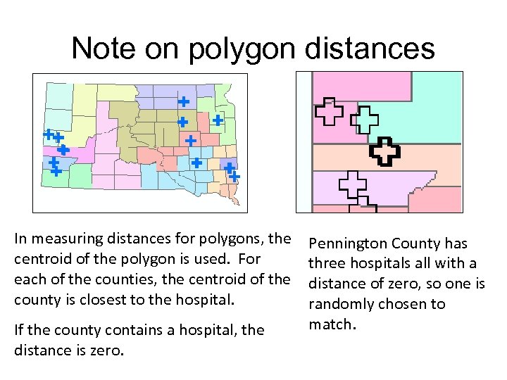Note on polygon distances In measuring distances for polygons, the centroid of the polygon is used. For each of the counties, the centroid of the county is closest to the hospital. If the county contains a hospital, the distance is zero. Pennington County has three hospitals all with a distance of zero, so one is randomly chosen to match.

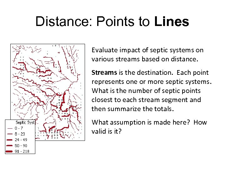Distance: Points to Lines Evaluate impact of septic systems on various streams based on distance. Streams is the destination. Each point represents one or more septic systems. What is the number of septic points closest to each stream segment and then summarize the totals. What assumption is made here? How valid is it?

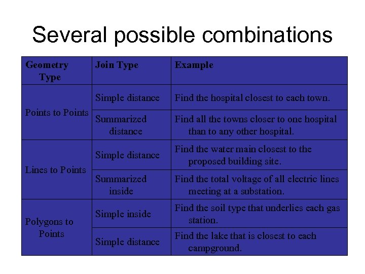Several possible combinations Geometry Type Polygons to Points Find the hospital closest to each town. Summarized distance Find all the towns closer to one hospital than to any other hospital. Simple distance Lines to Points Example Simple distance Points to Points Join Type Find the water main closest to the proposed building site. Summarized inside Find the total voltage of all electric lines meeting at a substation. Simple inside Find the soil type that underlies each gas station. Simple distance Find the lake that is closest to each campground.

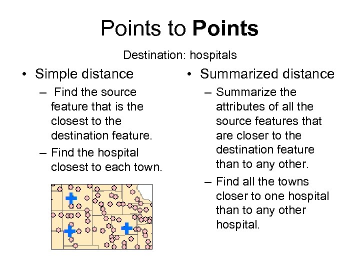Points to Points Destination: hospitals • Simple distance – Find the source feature that is the closest to the destination feature. – Find the hospital closest to each town. • Summarized distance – Summarize the attributes of all the source features that are closer to the destination feature than to any other. – Find all the towns closer to one hospital than to any other hospital.

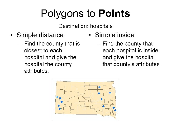Polygons to Points Destination: hospitals • Simple distance – Find the county that is closest to each hospital and give the hospital the county attributes. • Simple inside – Find the county that each hospital is inside and give the hospital that county’s attributes.

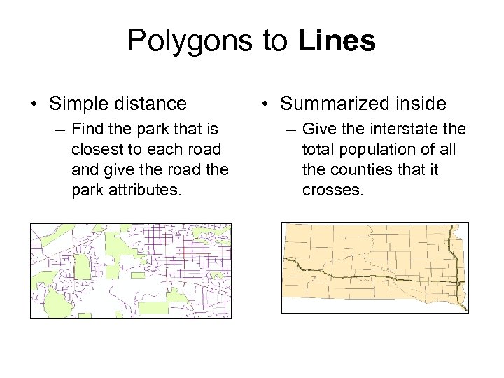Polygons to Lines • Simple distance – Find the park that is closest to each road and give the road the park attributes. • Summarized inside – Give the interstate the total population of all the counties that it crosses.

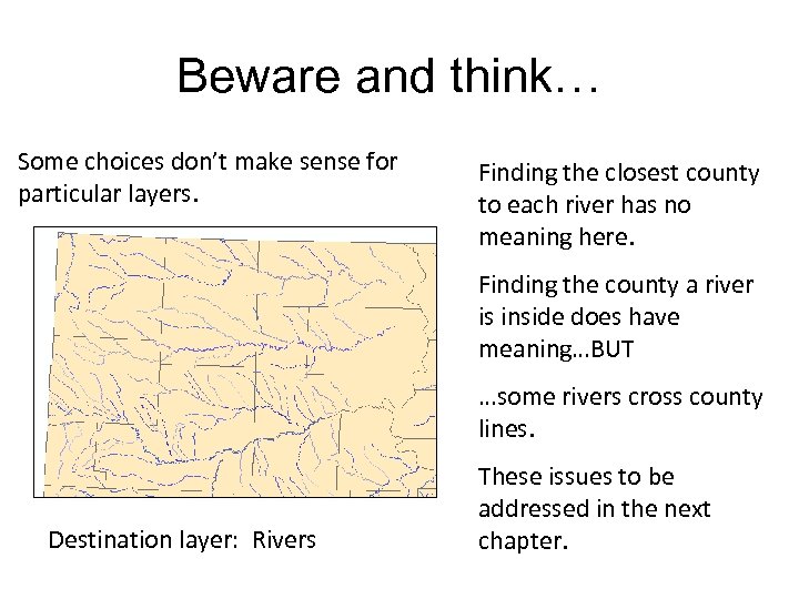Beware and think… Some choices don’t make sense for particular layers. Finding the closest county to each river has no meaning here. Finding the county a river is inside does have meaning…BUT …some rivers cross county lines. Destination layer: Rivers These issues to be addressed in the next chapter.

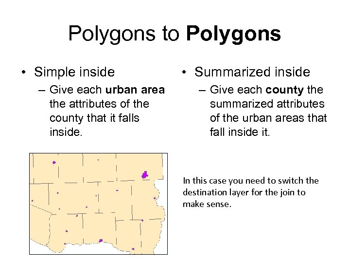Polygons to Polygons • Simple inside – Give each urban area the attributes of the county that it falls inside. • Summarized inside – Give each county the summarized attributes of the urban areas that fall inside it. In this case you need to switch the destination layer for the join to make sense.

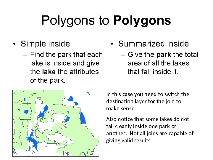Polygons to Polygons • Simple inside – Find the park that each lake is inside and give the lake the attributes of the park. • Summarized inside – Give the park the total area of all the lakes that fall inside it. In this case you need to switch the destination layer for the join to make sense. Also notice that some lakes do not fall cleanly inside one park or another. Not all joins are capable of giving valid results.

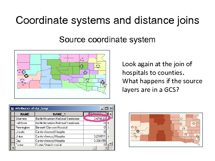Coordinate systems and distance joins Source coordinate system Look again at the join of hospitals to counties. What happens if the source layers are in a GCS?

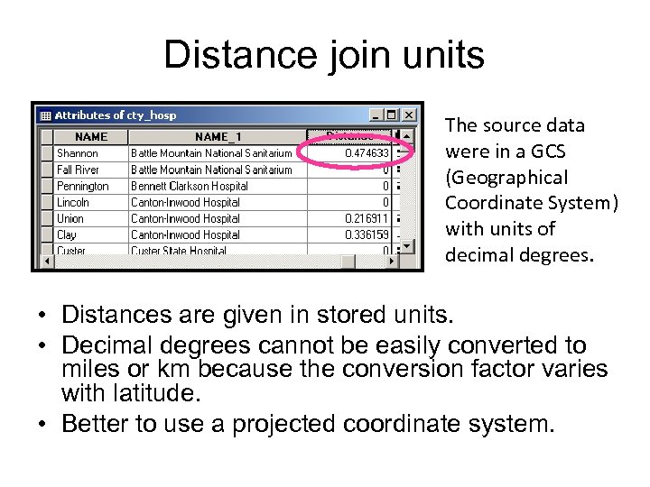Distance join units The source data were in a GCS (Geographical Coordinate System) with units of decimal degrees. • Distances are given in stored units. • Decimal degrees cannot be easily converted to miles or km because the conversion factor varies with latitude. • Better to use a projected coordinate system.

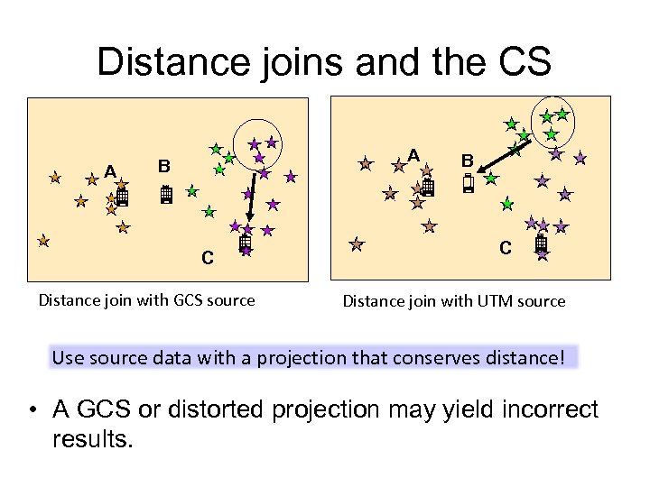Distance joins and the CS A A B C Distance join with GCS source B C Distance join with UTM source Use source data with a projection that conserves distance! • A GCS or distorted projection may yield incorrect results.

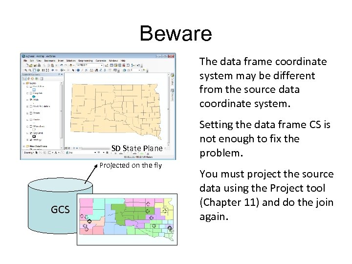Beware The data frame coordinate system may be different from the source data coordinate system. SD State Plane Projected on the fly GCS Setting the data frame CS is not enough to fix the problem. You must project the source data using the Project tool (Chapter 11) and do the join again.

References • Price, M. (2013). Mastering Arc. GIS (6 th ed. ). Mc. Graw-Hill. Mastering Arc. GIS, 6/e Instructor Edition Chapter 6: Power. Point Notes and Figures