Chapter 6 Sampling Distributions Where We ve Been

Chapter 6: Sampling Distributions

Where We’ve Been n The objective of most statistical analyses is inference. Sample statistics (mean, standard deviation) can be used to make decisions. Probability distributions can be used to construct models of populations. Mc. Clave: Statistics, 11 th ed. Chapter 6: Sampling Distributions 2

Where We’re Going n n n Develop the notion that sample statistic is a random variable with a probability distribution. Define a sampling distribution for a sample statistic. Link the sampling distribution of the sample mean to the normal distribution. Mc. Clave: Statistics, 11 th ed. Chapter 6: Sampling Distributions 3

n In practice, sample statistics are used to estimate population parameters. ¡ ¡ A parameter is a numerical descriptive measure of a population. Its value is almost always unknown. A sample statistic is a numerical descriptive measure of a sample. It can be calculated from the observations. Mc. Clave: Statistics, 11 th ed. Chapter 6: Sampling Distributions 4

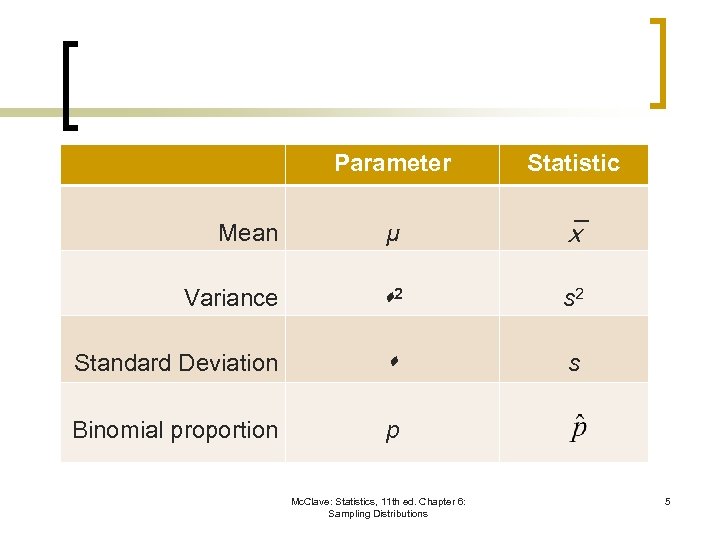
Parameter Statistic Mean µ Variance 2 s 2 Standard Deviation s Binomial proportion p Mc. Clave: Statistics, 11 th ed. Chapter 6: Sampling Distributions 5

6. 1: The Concept of a Sampling Distribution n n Since we could draw many different samples from a population, the sample statistic used to estimate the population parameter is itself a random variable. The probability distribution of a sample statistic calculated from a sample of n measurements is called the sampling distribution of the statistic. Mc. Clave: Statistics, 11 th ed. Chapter 6: Sampling Distributions 6

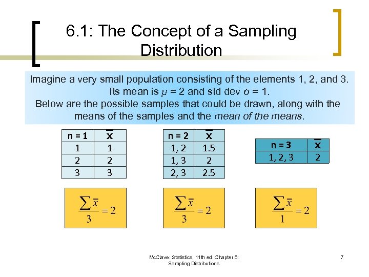
6. 1: The Concept of a Sampling Distribution Imagine a very small population consisting of the elements 1, 2, and 3. Its mean is μ = 2 and std dev σ = 1. Below are the possible samples that could be drawn, along with the means of the samples and the mean of the means. n=1 1 2 3 n=2 1, 3 2, 3 1. 5 2 2. 5 Mc. Clave: Statistics, 11 th ed. Chapter 6: Sampling Distributions n=3 1, 2, 3 2 7

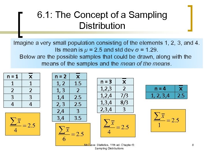
6. 1: The Concept of a Sampling Distribution Imagine a very small population consisting of the elements 1, 2, 3, and 4. Its mean is μ = 2. 5 and std dev σ = 1. 29. Below are the possible samples that could be drawn, along with the means of the samples and the mean of the means. n=1 1 2 3 4 n=2 1, 3 1, 4 2, 3 2, 4 3, 4 1. 5 2 2. 5 3 3. 5 n=3 1, 2, 4 1, 3, 4 2, 3, 4 2 7/3 8/3 3 Mc. Clave: Statistics, 11 th ed. Chapter 6: Sampling Distributions n=4 1, 2, 3, 4 2. 5 8

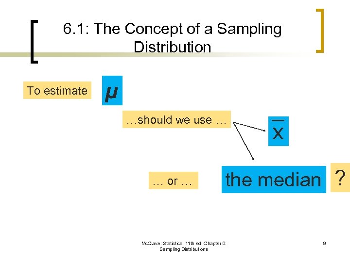
6. 1: The Concept of a Sampling Distribution To estimate µ …should we use … … or … the median ? Mc. Clave: Statistics, 11 th ed. Chapter 6: Sampling Distributions 9

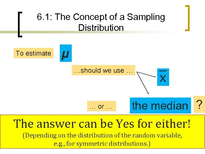
6. 1: The Concept of a Sampling Distribution To estimate µ …should we use … … or … the median ? The answer can be Yes for either! (Depending on the distribution of the random variable, Mc. Clave: Statistics, 11 th ed. Chapter e. g. , for symmetric. Distributions 6: distributions. ) Sampling 10

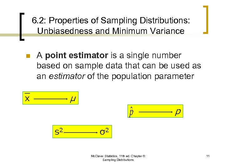
6. 2: Properties of Sampling Distributions: Unbiasedness and Minimum Variance n A point estimator is a single number based on sample data that can be used as an estimator of the population parameter µ p s 2 σ2 Mc. Clave: Statistics, 11 th ed. Chapter 6: Sampling Distributions 11

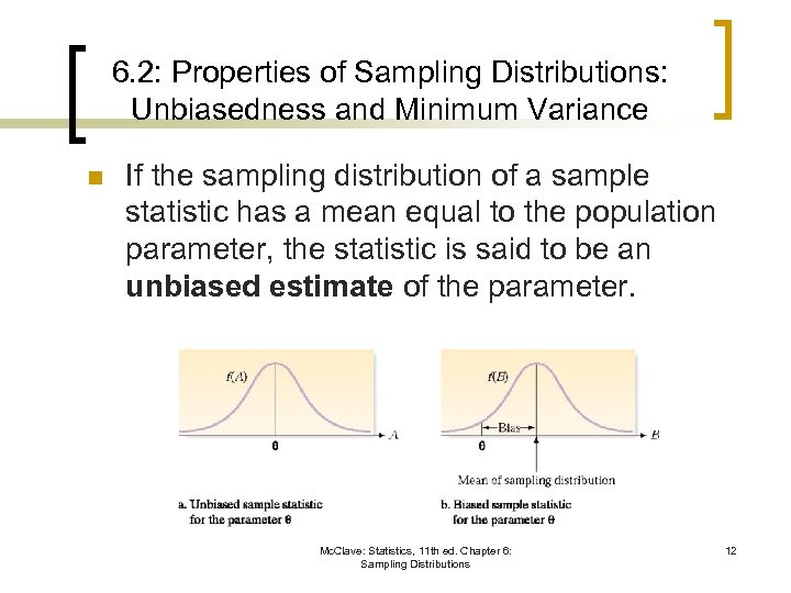
6. 2: Properties of Sampling Distributions: Unbiasedness and Minimum Variance n If the sampling distribution of a sample statistic has a mean equal to the population parameter, the statistic is said to be an unbiased estimate of the parameter. Mc. Clave: Statistics, 11 th ed. Chapter 6: Sampling Distributions 12

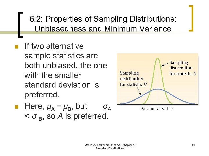
6. 2: Properties of Sampling Distributions: Unbiasedness and Minimum Variance n n If two alternative sample statistics are both unbiased, the one with the smaller standard deviation is preferred. Here, μA = μB, but σA < σ B, so A is preferred. Mc. Clave: Statistics, 11 th ed. Chapter 6: Sampling Distributions 13

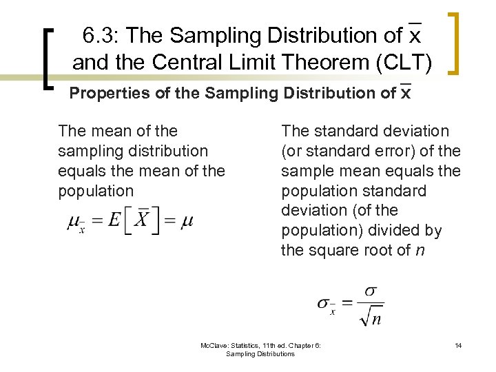
6. 3: The Sampling Distribution of and the Central Limit Theorem (CLT) Properties of the Sampling Distribution of The mean of the sampling distribution equals the mean of the population The standard deviation (or standard error) of the sample mean equals the population standard deviation (of the population) divided by the square root of n Mc. Clave: Statistics, 11 th ed. Chapter 6: Sampling Distributions 14

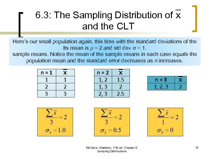
6. 3: The Sampling Distribution of and the CLT Here’s our small population again, this time with the standard deviations of the Its mean is μ = 2 and std dev σ = 1. sample means. Notice the mean of the sample means in each case equals the population mean and the standard error decreases as n increases. n=1 1 2 3 n=2 1, 3 2, 3 1. 5 2 2. 5 Mc. Clave: Statistics, 11 th ed. Chapter 6: Sampling Distributions n=3 1, 2, 3 2 15

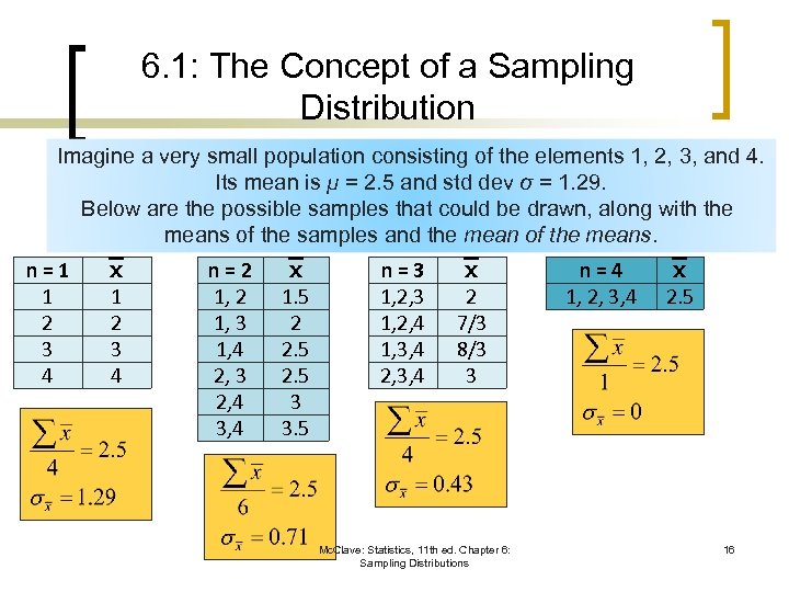
6. 1: The Concept of a Sampling Distribution Imagine a very small population consisting of the elements 1, 2, 3, and 4. Its mean is μ = 2. 5 and std dev σ = 1. 29. Below are the possible samples that could be drawn, along with the means of the samples and the mean of the means. n=1 1 2 3 4 n=2 1, 3 1, 4 2, 3 2, 4 3, 4 1. 5 2 2. 5 3 3. 5 n=3 1, 2, 4 1, 3, 4 2, 3, 4 2 7/3 8/3 3 Mc. Clave: Statistics, 11 th ed. Chapter 6: Sampling Distributions n=4 1, 2, 3, 4 2. 5 16

6. 3: The Sampling Distribution of and the CLT n If a random sample of n observations is drawn from a normally distributed population, the sampling distribution of will be normally distributed Mc. Clave: Statistics, 11 th ed. Chapter 6: Sampling Distributions 17

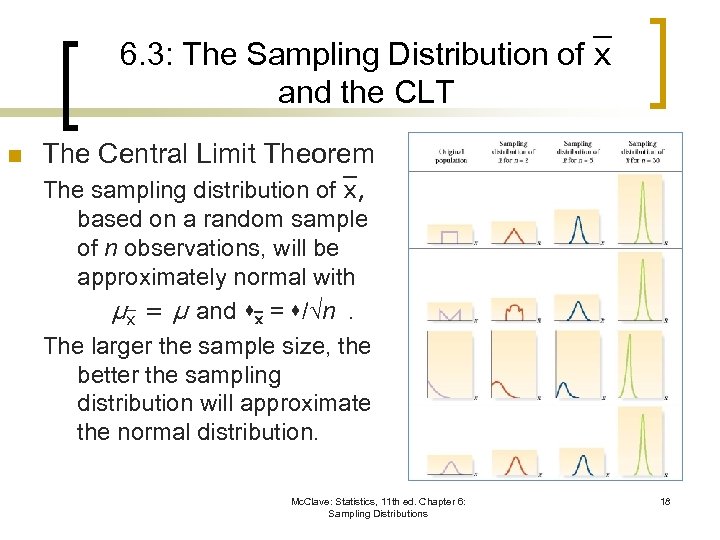
6. 3: The Sampling Distribution of and the CLT n The Central Limit Theorem The sampling distribution of , based on a random sample of n observations, will be approximately normal with µ = µ and = /√n. The larger the sample size, the better the sampling distribution will approximate the normal distribution. Mc. Clave: Statistics, 11 th ed. Chapter 6: Sampling Distributions 18

6. 3: The Sampling Distribution of and the CLT Suppose existing houses for sale average 2200 square meter in size, with a standard deviation of 250 m 2. What is the probability that a randomly selected sample of 36 houses will average at least 2300 m 2 ? Mc. Clave: Statistics, 11 th ed. Chapter 6: Sampling Distributions 19

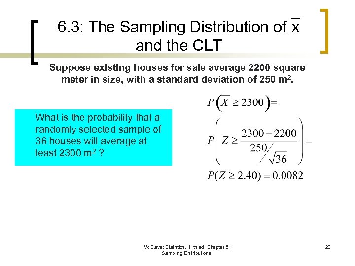
6. 3: The Sampling Distribution of and the CLT Suppose existing houses for sale average 2200 square meter in size, with a standard deviation of 250 m 2. What is the probability that a randomly selected sample of 36 houses will average at least 2300 m 2 ? Mc. Clave: Statistics, 11 th ed. Chapter 6: Sampling Distributions 20

6. 3: The Sampling Distribution of and the CLT Suppose existing houses for sale average 2200 square meter in size, with a standard deviation of 250 m 2. Assuming the areas of the house are normal, what is the probability that a randomly selected house will have at least 2300 m 2 ? Mc. Clave: Statistics, 11 th ed. Chapter 6: Sampling Distributions 21

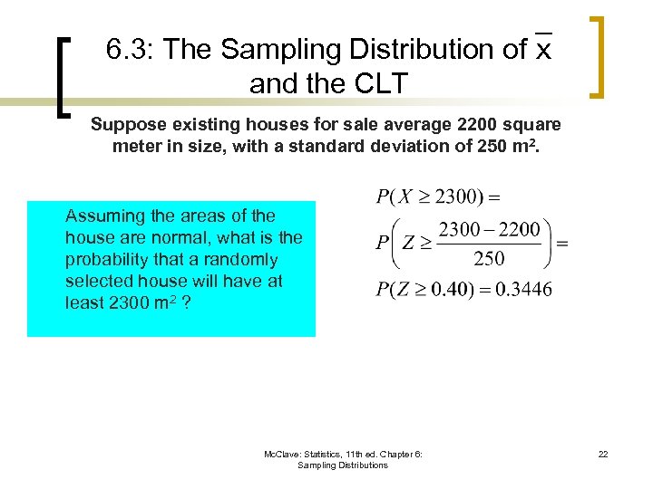
6. 3: The Sampling Distribution of and the CLT Suppose existing houses for sale average 2200 square meter in size, with a standard deviation of 250 m 2. Assuming the areas of the house are normal, what is the probability that a randomly selected house will have at least 2300 m 2 ? Mc. Clave: Statistics, 11 th ed. Chapter 6: Sampling Distributions 22

6. 3: The Sampling Distribution of and the CLT Suppose existing houses for sale average 2200 square meter in size, with a standard deviation of 250 m 2. (1) Assuming the areas of the house are normal, what is the probability that a randomly selected house will have at least 2300 m 2 ? (2) What is the probability that a randomly selected sample of 36 houses will average at least 2300 m 2 ? Notice that in (1) we assumed normality of the areas of the houses, but in (2) we do not need to assume this, because n=36>30 so by CLT the average of 36 houses is approximately normal. Mc. Clave: Statistics, 11 th ed. Chapter 6: Sampling Distributions 23