Chapter 6 Efficient Diversification.pptx
- Количество слайдов: 44
Chapter 6: “Efficient Diversification” Source Book: Essentials of Investment, 7 th edition. Investment Zvi Bodie, Alex Kane, Alan J. Marcus Prepared by: Ilyas Imachikov
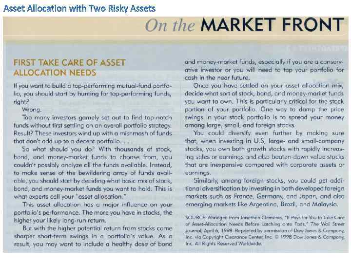
Market Risk VS Firm-specific Risk Market (systematic/nondiversifiable) risk • Risk factors common to the whole economy. • Example: • General economic conditions in local economy or industry • General economic, political, social factors and conditions • General economic/industry-wide cataclysms • Storms, earthquakes, other catastrophes • Wars, or civil conflicts • Etc. Firm-specific (nonsystematic/diversifiable/unique) risk • Risk factors attributable only to particular firm or security. • Risk that can be eliminated by diversification • Example: • All inside factors attributable to a firm • Firm-specific competences and endowments • Good or bad management • Firm-specific cataclysms • Death of a major CEO • Accidents during production • Bad risk or security management • Etc.
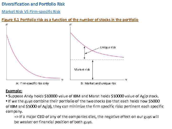
Market Risk VS Firm-specific Risk Figure 6. 1 Portfolio risk as a function of the number of stocks in the portfolio Example: • Suppose Andy holds $10000 value of IBM and Marat holds $10000 value of Agip stock. • If we the guys combine their portfolio of the two stocks (so that each holds now $5000 of IBM and $5000 of Agip), they can minimize the firm specific risks pertinent each specific company. => If a major CEO of any of the companies dies, the negative effect on our guys will be weaker on financial position of both guys.
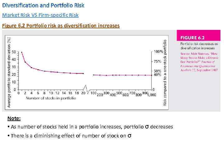
Market Risk VS Firm-specific Risk Figure 6. 2 Portfolio risk as diversification increases Note: • As number of stocks held in a portfolio increases, portfolio σ decreases • There is a diminishing effect of number of stock on σ
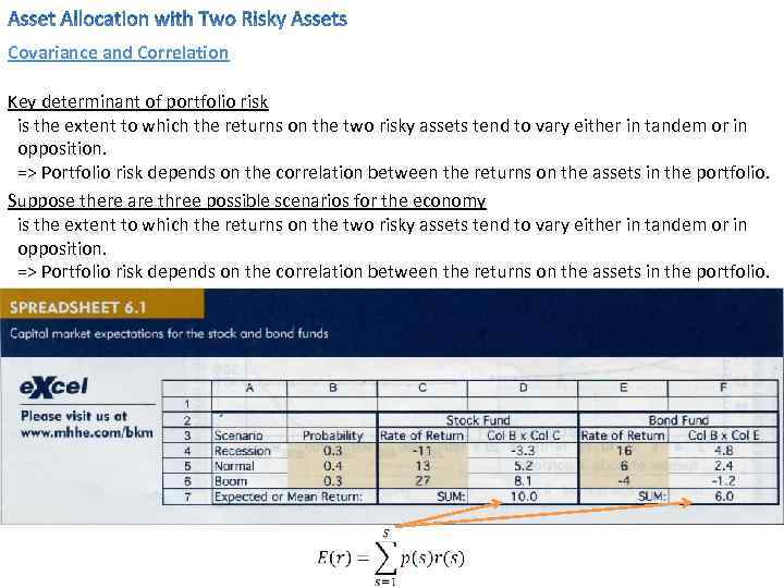
Covariance and Correlation Key determinant of portfolio risk is the extent to which the returns on the two risky assets tend to vary either in tandem or in opposition. => Portfolio risk depends on the correlation between the returns on the assets in the portfolio. Suppose there are three possible scenarios for the economy is the extent to which the returns on the two risky assets tend to vary either in tandem or in opposition. => Portfolio risk depends on the correlation between the returns on the assets in the portfolio.
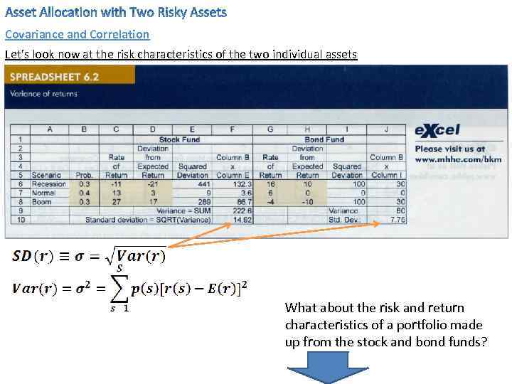
Covariance and Correlation Let’s look now at the risk characteristics of the two individual assets What about the risk and return characteristics of a portfolio made up from the stock and bond funds?
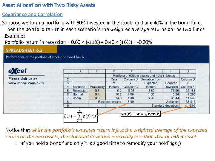
Covariance and Correlation Suppose we form a portfolio with 60% invested in the stock fund and 40% in the bond fund. Then the portfolio return in each scenario is the weighted average returns on the two funds Example: Portfolio return in recession = 0. 60 × (-11%) + 0. 40 × (16%) = -0. 20% Notice that while the portfolio’s expected return is just the weighted average of the expected return on the two assets, the standard deviation is actually less than that of either asset. ÞIf you hold a bond fund only it is a good time to remodify your holdings ; )
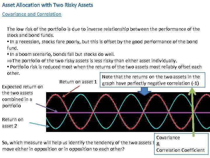
Covariance and Correlation The low risk of the portfolio is due to inverse relationship between the performance of the stock and bond funds. • In a recession, stocks fare poorly, but this is offset by the good performance of the bond fund. • In a boom scenario, bonds fall but stocks do well. ÞThe portfolio of the two risky assets is less risky than either asset individually. • Portfolio risk is reduced most when the returns of the two assets most reliably offset each other. Note that the returns on the two assets in the Return on asset 1 graph have perfectly negative correlation (-1) Expected return on the two assets combined in a portfolio Return on asset 2 Covariance So, which measure will help us identify the tendency of the two assets to& move either in opposition or in opposition to each other? Correlation Coefficient
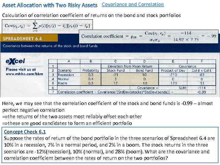
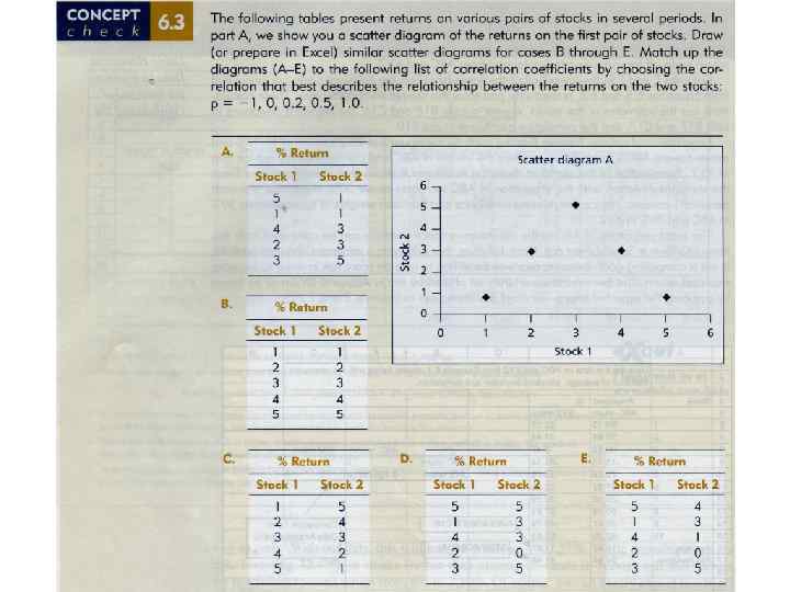
Covariance and Correlation Calculation of correlation coefficient of returns on the bond and stock portfolios Here, we may see that the correlation coefficient of the stock and bond funds is -0. 99 – almost perfect negative correlation Þthe returns of the two assets most reliably offset each other Þthese are good candidates to form an efficient portfolio Concept Check 6. 1 Suppose the rates of return of the bond portfolio in the three scenarios of Spreadsheet 6. 4 are 10% in a recession, 7% in a normal period, and 2% in a boom. The stock returns in the three scenarios are -12%(recession), 10% (normal), and 28% (boom). What are the covariance and correlation coefficient between the rates of return on the two portfolios?
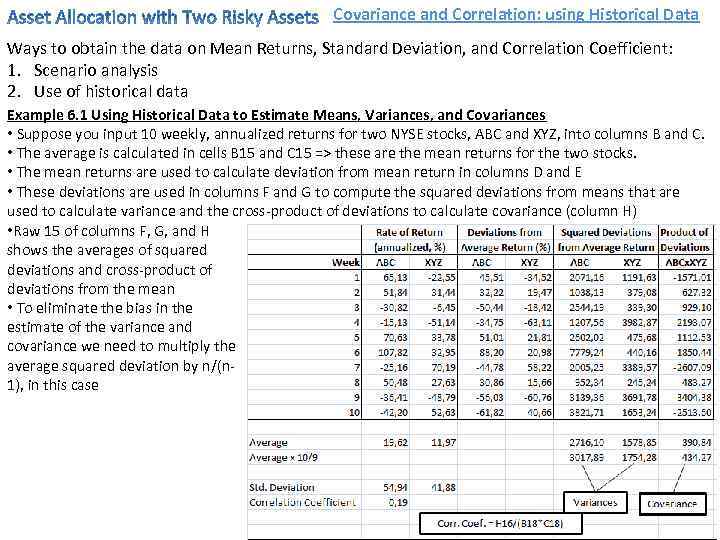
Covariance and Correlation: using Historical Data Ways to obtain the data on Mean Returns, Standard Deviation, and Correlation Coefficient: 1. Scenario analysis 2. Use of historical data Example 6. 1 Using Historical Data to Estimate Means, Variances, and Covariances • Suppose you input 10 weekly, annualized returns for two NYSE stocks, ABC and XYZ, into columns B and C. • The average is calculated in cells B 15 and C 15 => these are the mean returns for the two stocks. • The mean returns are used to calculate deviation from mean return in columns D and E • These deviations are used in columns F and G to compute the squared deviations from means that are used to calculate variance and the cross-product of deviations to calculate covariance (column H) • Raw 15 of columns F, G, and H shows the averages of squared deviations and cross-product of deviations from the mean • To eliminate the bias in the estimate of the variance and covariance we need to multiply the average squared deviation by n/(n 1), in this case
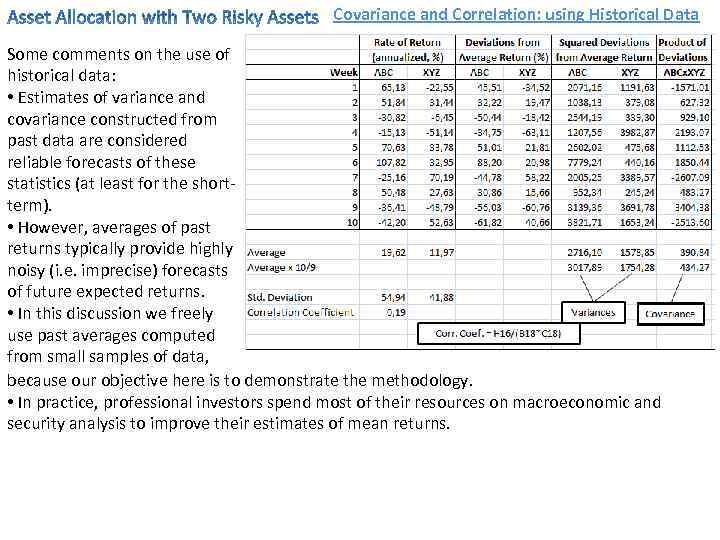
Covariance and Correlation: using Historical Data Some comments on the use of historical data: • Estimates of variance and covariance constructed from past data are considered reliable forecasts of these statistics (at least for the shortterm). • However, averages of past returns typically provide highly noisy (i. e. imprecise) forecasts of future expected returns. • In this discussion we freely use past averages computed from small samples of data, because our objective here is to demonstrate the methodology. • In practice, professional investors spend most of their resources on macroeconomic and security analysis to improve their estimates of mean returns.
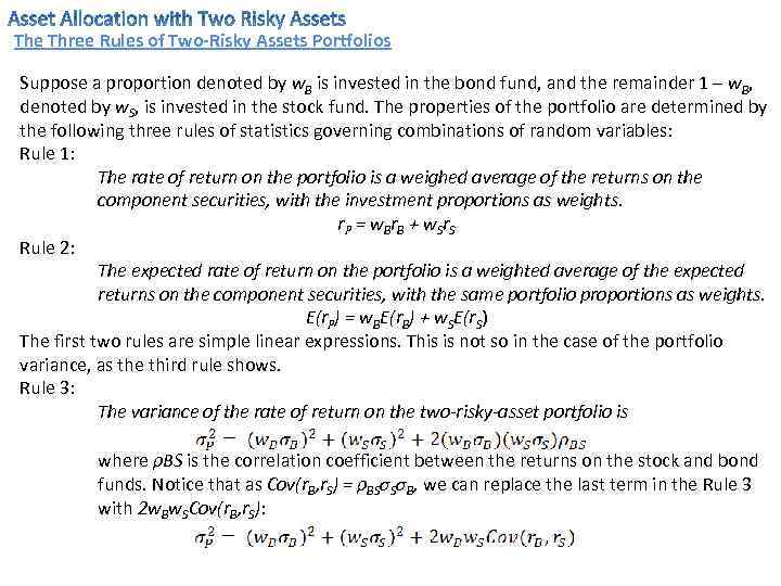
The Three Rules of Two-Risky Assets Portfolios Suppose a proportion denoted by w. B is invested in the bond fund, and the remainder 1 – w. B, denoted by w. S, is invested in the stock fund. The properties of the portfolio are determined by the following three rules of statistics governing combinations of random variables: Rule 1: The rate of return on the portfolio is a weighed average of the returns on the component securities, with the investment proportions as weights. r P = w B r B + w Sr S Rule 2: The expected rate of return on the portfolio is a weighted average of the expected returns on the component securities, with the same portfolio proportions as weights. E(r. P) = w. BE(r. B) + w. SE(r. S) The first two rules are simple linear expressions. This is not so in the case of the portfolio variance, as the third rule shows. Rule 3: The variance of the rate of return on the two-risky-asset portfolio is where ρBS is the correlation coefficient between the returns on the stock and bond funds. Notice that as Cov(r. B, r. S) = ρBSσSσB, we can replace the last term in the Rule 3 with 2 w. Bw. SCov(r. B, r. S):
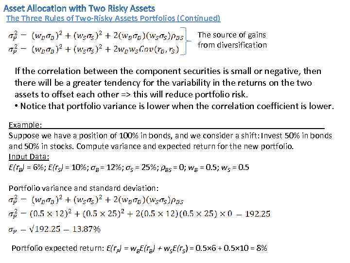
The Three Rules of Two-Risky Assets Portfolios (Continued) The source of gains from diversification If the correlation between the component securities is small or negative, then there will be a greater tendency for the variability in the returns on the two assets to offset each other => this will reduce portfolio risk. • Notice that portfolio variance is lower when the correlation coefficient is lower. Example: _________________________________ Suppose we have a position of 100% in bonds, and we consider a shift: Invest 50% in bonds and 50% in stocks. Compute variance and expected return for the new portfolio. Input Data: E(r. B) = 6%; E(r. S) = 10%; σB = 12%; σS = 25%; ρBS = 0; w. B = 0. 5; w. S = 0. 5 Portfolio variance and standard deviation: Portfolio expected return: E(r. P) = w. BE(r. B) + w. SE(r. S) = 0. 5× 6 + 0. 5× 10 = 8%
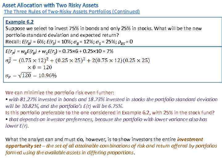
The Three Rules of Two-Risky Assets Portfolios (Continued) Example 6. 2 Suppose we select to invest 75% in bonds and only 25% in stocks. What will be the new portfolio standard deviation and expected return? Recall: E(r. B) = 6%; E(r. S) = 10%; σB = 12%; σS = 25%; ρBS = 0 E(r. P) = w. BE(r. B) + w. SE(r. S) = 0. 75× 6 + 0. 25× 10 = 7% We can minimize the portfolio risk even further: • with 81. 27% invested in bonds and 18. 73% invested in stocks the portfolio standard deviation will be 10. 82%, and the portfolio’s E(r) will be 6. 75%. Is this portfolio preferable to the one considered in Example 6. 2, with 25% in the stock fund? • that depends on investor preferences, because the portfolio with lower variance also has lower E(r). What the analyst can and must do, however, is to show investors the entire investment opportunity set – the set of all attainable combinations of risk and return offered by portfolios formed using the available assets in differing proportions.
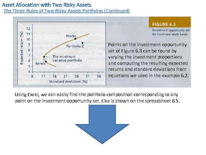
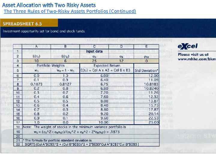
The Three Rules of Two-Risky Assets Portfolios (Continued) Points on the investment opportunity set of Figure 6. 3 can be found by varying the investment proportions and computing the resulting expected returns and standard deviations from equations we used in the example 6. 2. Using Excel, we can easily find the portfolio composition corresponding to any point on the investment opportunity set. Like is shown on the spreadsheet 6. 5.
The Three Rules of Two-Risky Assets Portfolios (Continued)
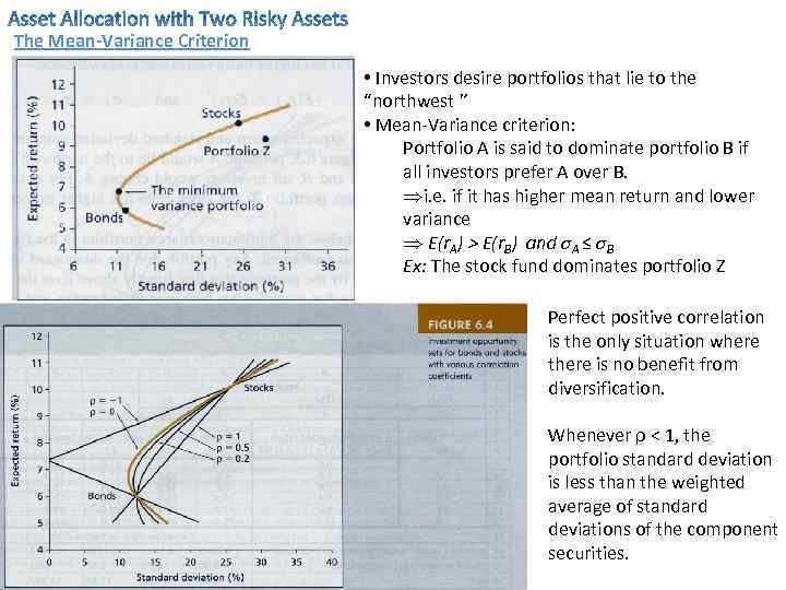
The Mean-Variance Criterion • Investors desire portfolios that lie to the “northwest ” • Mean-Variance criterion: Portfolio A is said to dominate portfolio B if all investors prefer A over B. Þi. e. if it has higher mean return and lower variance Þ E(r. A) > E(r. B) and σA ≤ σB Ex: The stock fund dominates portfolio Z Perfect positive correlation is the only situation where there is no benefit from diversification. Whenever ρ < 1, the portfolio standard deviation is less than the weighted average of standard deviations of the component securities.
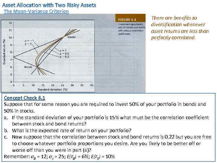
The Mean-Variance Criterion There are benefits to diversification whenever asset returns are less than perfectly correlated. Concept Check 6. 1 Suppose that for some reason you are required to invest 50% of your portfolio in bonds and 50% in stocks. a. If the standard deviation of your portfolio is 15% what must be the correlation coefficient between stock and bond returns? b. What is the expected rate of return on your portfolio? c. Now suppose that the correlation between stock and bond returns is 0. 22 but you are free to choose whatever portfolio proportions you desire. Are you likely to be better off or worse off than you were in part (a)? Remember: σB = 12; σs = 25; E(r. B) = 6%; E(r. S) = 10%
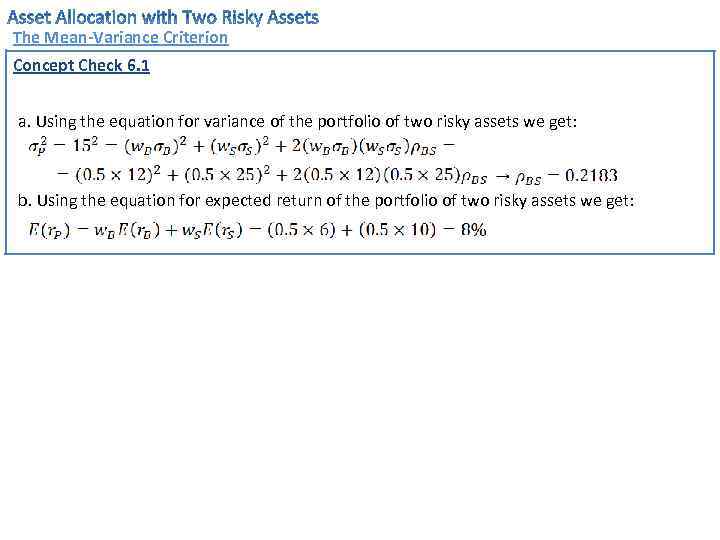
The Mean-Variance Criterion Concept Check 6. 1 a. Using the equation for variance of the portfolio of two risky assets we get: b. Using the equation for expected return of the portfolio of two risky assets we get:
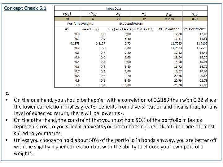
Concept Check 6. 1 c. • On the one hand, you should be happier with a correlation of 0. 2183 than with 0. 22 since the lower correlation implies greater benefits from diversification and means that, for any level of expected return, there will be lower risk. • On the other hand, the constraint that you must hold 50% of the portfolio in bonds represents cost to you since it prevents you from choosing the risk-return trade-off most suited to your tastes. • Unless you choose to hold about 50% of the portfolio in bonds anyway, you are better off with the slightly higher correlation but with the ability to choose your own portfolio weights.

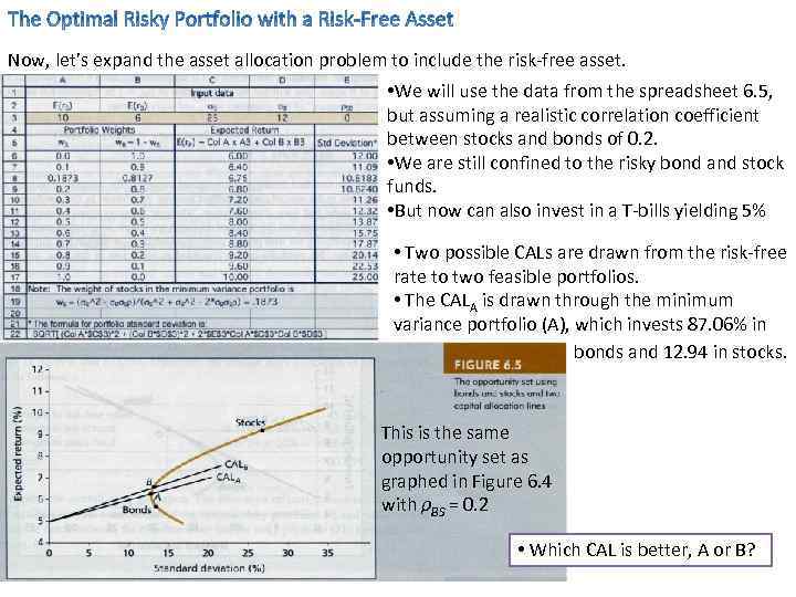
Now, let’s expand the asset allocation problem to include the risk-free asset. • We will use the data from the spreadsheet 6. 5, but assuming a realistic correlation coefficient between stocks and bonds of 0. 2. • We are still confined to the risky bond and stock funds. • But now can also invest in a T-bills yielding 5% • Two possible CALs are drawn from the risk-free rate to two feasible portfolios. • The CALA is drawn through the minimum variance portfolio (A), which invests 87. 06% in bonds and 12. 94 in stocks. This is the same opportunity set as graphed in Figure 6. 4 with ρBS = 0. 2 • Which CAL is better, A or B?
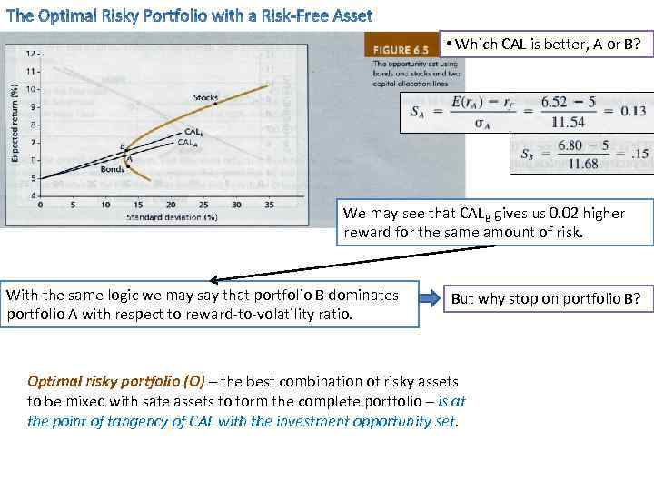
• Which CAL is better, A or B? We may see that CALB gives us 0. 02 higher reward for the same amount of risk. With the same logic we may say that portfolio B dominates portfolio A with respect to reward-to-volatility ratio. But why stop on portfolio B? Optimal risky portfolio (O) – the best combination of risky assets to be mixed with safe assets to form the complete portfolio – is at the point of tangency of CAL with the investment opportunity set.
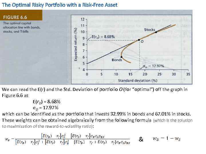
We can read the E(r) and the Std. Deviation of portfolio O (for “optimal”) off the graph in Figure 6. 6 as E(r. O) = 8. 68% σO = 17. 97% which can be identified as the portfolio that invests 32. 99% in bonds and 67. 01% in stocks. These weights can be obtained algebraically from the following formula (which is the solution to maximization of the reward-to-volatility ratio): &
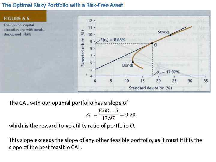
The CAL with our optimal portfolio has a slope of which is the reward-to-volatility ratio of portfolio O. This slope exceeds the slope of any other feasible portfolio, as it must if it is the slope of the best feasible CAL.
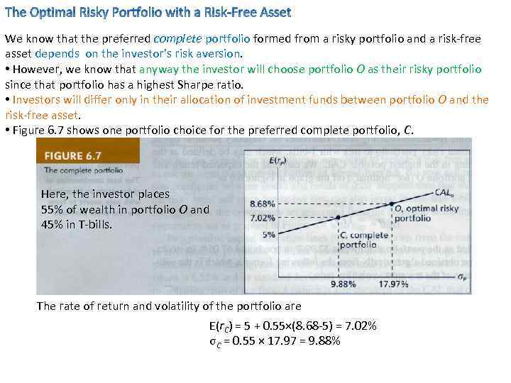
We know that the preferred complete portfolio formed from a risky portfolio and a risk-free asset depends on the investor’s risk aversion. • However, we know that anyway the investor will choose portfolio O as their risky portfolio since that portfolio has a highest Sharpe ratio. • Investors will differ only in their allocation of investment funds between portfolio O and the risk-free asset. • Figure 6. 7 shows one portfolio choice for the preferred complete portfolio, C. Here, the investor places 55% of wealth in portfolio O and 45% in T-bills. The rate of return and volatility of the portfolio are E(r. C) = 5 + 0. 55×(8. 68 -5) = 7. 02% σC = 0. 55 × 17. 97 = 9. 88%
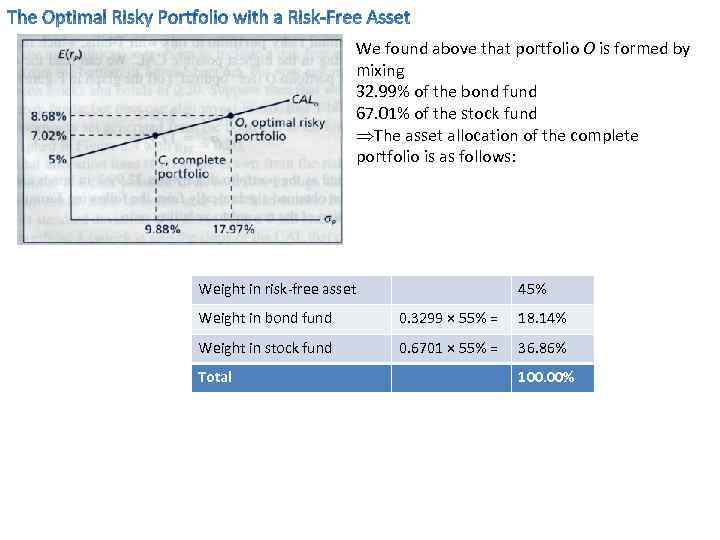
We found above that portfolio O is formed by mixing 32. 99% of the bond fund 67. 01% of the stock fund ÞThe asset allocation of the complete portfolio is as follows: Weight in risk-free asset 45% Weight in bond fund 0. 3299 × 55% = 18. 14% Weight in stock fund 0. 6701 × 55% = 36. 86% Total 100. 00%
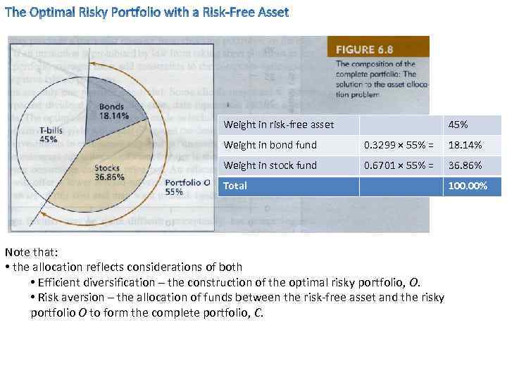
Weight in risk-free asset 45% Weight in bond fund 0. 3299 × 55% = 18. 14% Weight in stock fund 0. 6701 × 55% = 36. 86% Total Note that: • the allocation reflects considerations of both • Efficient diversification – the construction of the optimal risky portfolio, O. • Risk aversion – the allocation of funds between the risk-free asset and the risky portfolio O to form the complete portfolio, C. 100. 00%
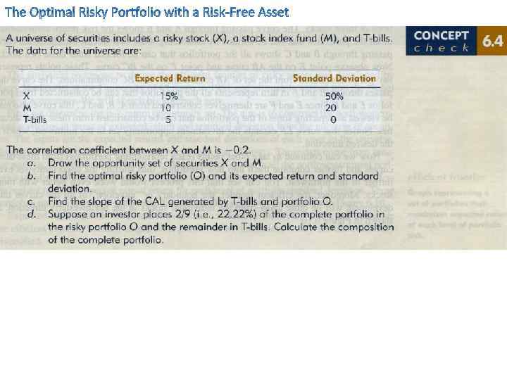
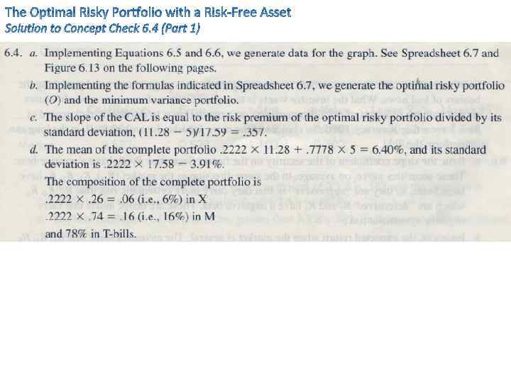
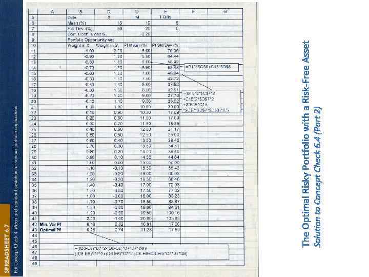
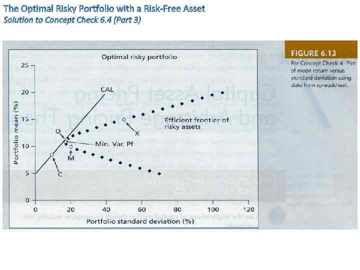
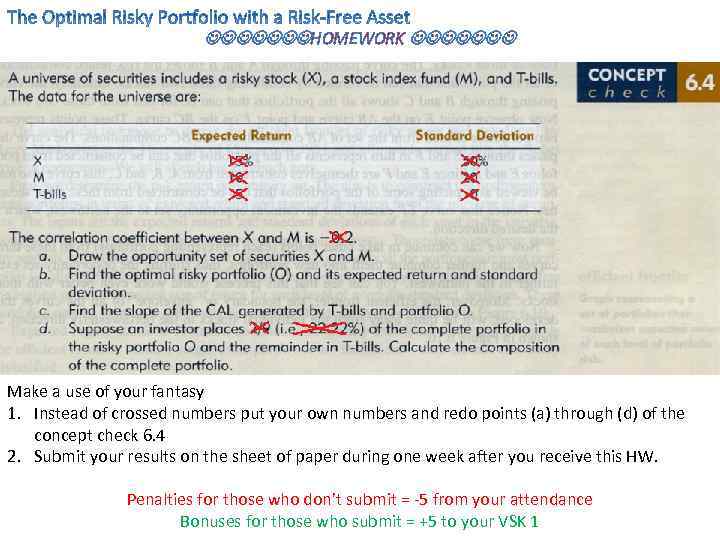
HOMEWORK Make a use of your fantasy 1. Instead of crossed numbers put your own numbers and redo points (a) through (d) of the concept check 6. 4 2. Submit your results on the sheet of paper during one week after you receive this HW. Penalties for those who don’t submit = -5 from your attendance Bonuses for those who submit = +5 to your VSK 1
Factor Model – statistical model to measure the firm-specific versus systematic risk of a stock’s rate of return. To construct the efficient frontier from a universe of 100 securities we would need to estimate • 100 expected returns • 100 variances • 100× 99/2 = 4’ 950 covariances And a universe of 100 securities is small! The assumption that one common factor (or we can say one set of common factors) is responsible for all the covariability of stock returns, with all other variability due to firmspecific factors, dramatically simplifies the analysis. Excess return – rate of return in excess of the risk-free rate. Ri = ri - rf We can express the distinction between macroeconomic and firm-specific factors by decomposing this excess return in some holding period into three components Ri = E(Ri) + βi. M + ei where E(Ri) is the excess expected HPR at the start of the holding period M is the market or economic surprise factor β is the sensitivity of the security to the macroeconomic factor ei is the impact of unanticipated firm-specific events
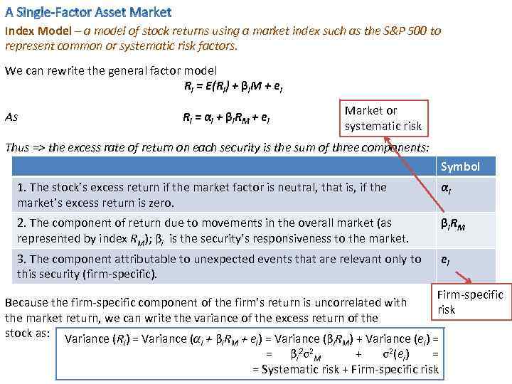
Index Model – a model of stock returns using a market index such as the S&P 500 to represent common or systematic risk factors. We can rewrite the general factor model Ri = E(Ri) + βi. M + ei As Market or systematic risk Ri = αi + βi. RM + ei Thus => the excess rate of return on each security is the sum of three components: Symbol 1. The stock’s excess return if the market factor is neutral, that is, if the market’s excess return is zero. αi 2. The component of return due to movements in the overall market (as represented by index RM); βi is the security’s responsiveness to the market. βi. RM 3. The component attributable to unexpected events that are relevant only to this security (firm-specific). ei Firm-specific Because the firm-specific component of the firm’s return is uncorrelated with risk the market return, we can write the variance of the excess return of the stock as: Variance (R ) = Variance (α + β R + e ) = Variance (β R ) + Variance (e ) = i i i M i βi 2σ2 M i M σ2(ei) i = + = = Systematic risk + Firm-specific risk
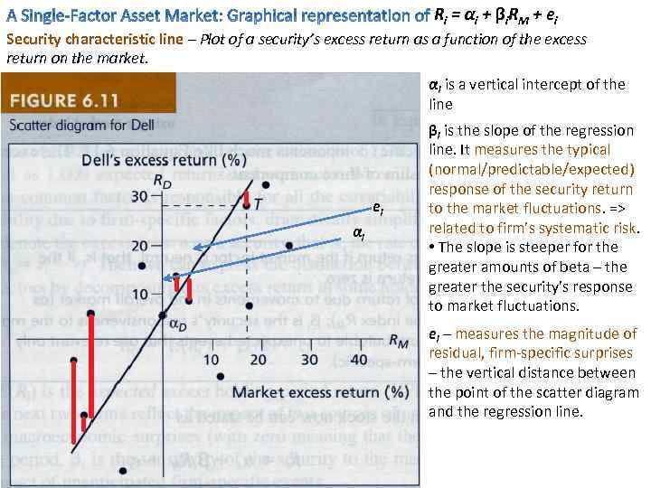
R i = αi + βi R M + ei Security characteristic line – Plot of a security’s excess return as a function of the excess return on the market. αi is a vertical intercept of the line ei αi βi is the slope of the regression line. It measures the typical (normal/predictable/expected) response of the security return to the market fluctuations. => related to firm’s systematic risk. • The slope is steeper for the greater amounts of beta – the greater the security’s response to market fluctuations. ei – measures the magnitude of residual, firm-specific surprises – the vertical distance between the point of the scatter diagram and the regression line.
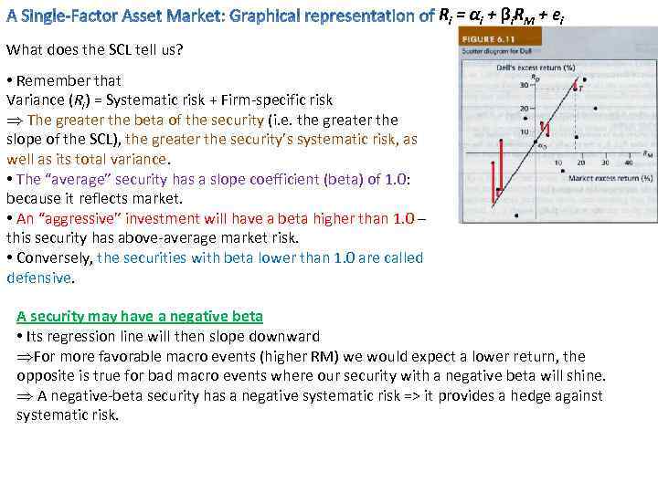
R i = αi + βi R M + ei What does the SCL tell us? • Remember that Variance (Ri) = Systematic risk + Firm-specific risk Þ The greater the beta of the security (i. e. the greater the slope of the SCL), the greater the security’s systematic risk, as well as its total variance. • The “average” security has a slope coefficient (beta) of 1. 0: because it reflects market. • An “aggressive” investment will have a beta higher than 1. 0 – this security has above-average market risk. • Conversely, the securities with beta lower than 1. 0 are called defensive. A security may have a negative beta • Its regression line will then slope downward ÞFor more favorable macro events (higher RM) we would expect a lower return, the opposite is true for bad macro events where our security with a negative beta will shine. Þ A negative-beta security has a negative systematic risk => it provides a hedge against systematic risk.
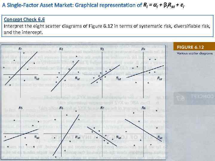
R i = αi + βi R M + ei Concept Check 6. 6 Interpret the eight scatter diagrams of Figure 6. 12 in terms of systematic risk, diversifiable risk, and the intercept.
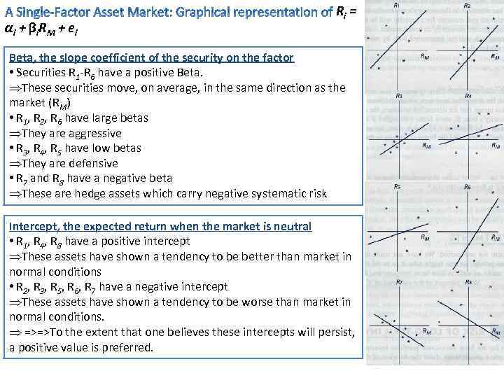
αi + βi R M + ei Ri = Beta, the slope coefficient of the security on the factor • Securities R 1 -R 6 have a positive Beta. ÞThese securities move, on average, in the same direction as the market (RM) • R 1, R 2, R 6 have large betas ÞThey are aggressive • R 3, R 4, R 5 have low betas ÞThey are defensive • R 7 and R 8 have a negative beta ÞThese are hedge assets which carry negative systematic risk Intercept, the expected return when the market is neutral • R 1, R 4, R 8 have a positive intercept ÞThese assets have shown a tendency to be better than market in normal conditions • R 2, R 3, R 5, R 6, R 7 have a negative intercept ÞThese assets have shown a tendency to be worse than market in normal conditions. Þ =>=>To the extent that one believes these intercepts will persist, a positive value is preferred.
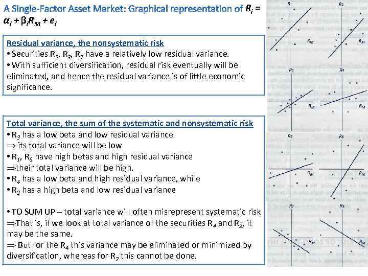
αi + βi R M + ei Ri = Residual variance, the nonsystematic risk • Securities R 2, R 3, R 7 have a relatively low residual variance. • With sufficient diversification, residual risk eventually will be eliminated, and hence the residual variance is of little economic significance. Total variance, the sum of the systematic and nonsystematic risk • R 3 has a low beta and low residual variance Þ its total variance will be low • R 1, R 6 have high betas and high residual variance Þtheir total variance will be high. • R 4 has a low beta and high residual variance, while • R 2 has a high beta and low residual variance • TO SUM UP – total variance will often misrepresent systematic risk ÞThat is, if we look at total variance of the securities R 4 and R 2, it may be the same. Þ But for the R 4 this variance may be eliminated or minimized by diversification, whereas for R 2 this cannot be done.
How to identify beta: Example 6. 4, page 176
Chapter 6 Efficient Diversification.pptx