

f12cc37bf489f0f1e7eb428c081ead97.ppt
- Количество слайдов: 39
 • Chapter 6 Demand • Key Concept: the demand function x 1 (p 1, p 2, m) • Income m: normal good, inferior good • Own price p 1: Giffen good, ordinary good • Other price p 2: substitute, complement
 • Chapter 6 Demand • The demand function gives the optimal amounts of each of the goods as a function of the prices and income faced by the consumer: x 1 (p 1, p 2, m) • We now change the arguments in the demand function one by one.
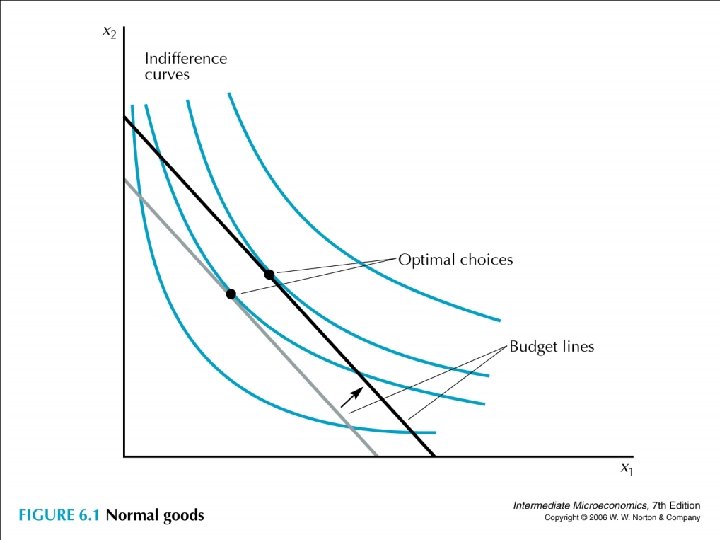
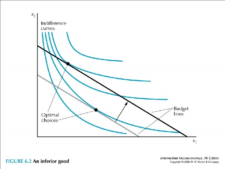
 • ∆x 1/∆m > 0: good 1 is a normal good ∆x 1/∆m < 0: good 1 is an inferior good • It depends on the income level we are talking about (bus, MRT, taxi).
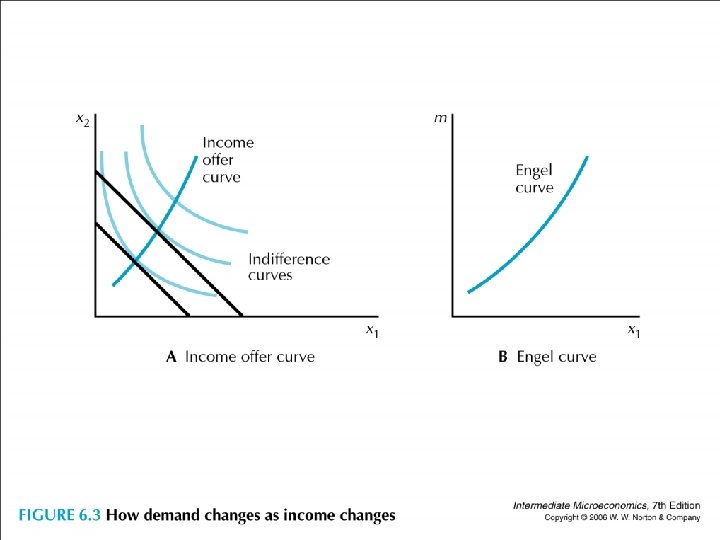
 At x") • Two ways to look at the same thing • (1) At x 1 – x 2 space, connect the demanded bundles as the budget line gets shifted outward. This curve is called the income offer curve (IOC) or income expansion path. • (2) At x 1 – m space, connect the optimal x 1 bundles as the income increases while holding all prices fixed. This curve is called the Engel curve.
• Two ways to look at the same thing • (1) At x 1 – x 2 space, connect the demanded bundles as the budget line gets shifted outward. This curve is called the income offer curve (IOC) or income expansion path. • (2) At x 1 – m space, connect the optimal x 1 bundles as the income increases while holding all prices fixed. This curve is called the Engel curve.
 • Draw a general preference to illustrate the income offer curve and the Engel curve.
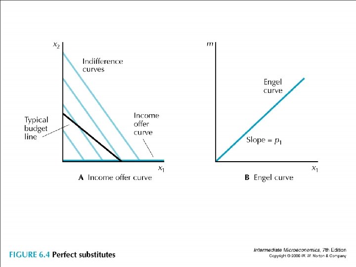
 • Look at specific preferences. • Perfect substitutes: p 1 < p 2, IOC (x axis) Engel (sloped p 1) think about p 1 > p 2 and p 1 = p 2.
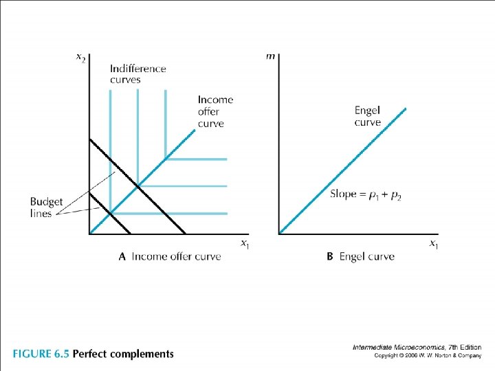
 Engel (sloped p 1+ p 2)") • Perfect complements: IOC (at the corner) Engel (sloped p 1+ p 2)
• Perfect complements: IOC (at the corner) Engel (sloped p 1+ p 2)
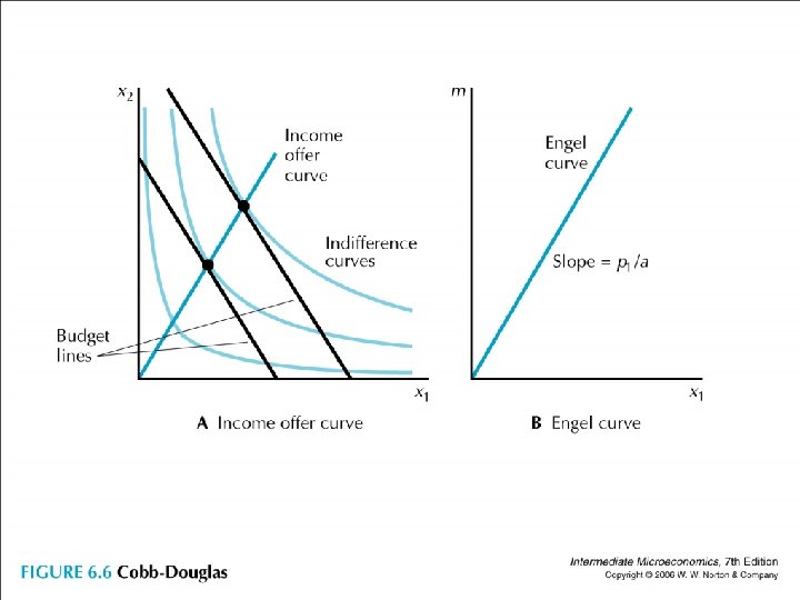
 • Cobb-Douglas: x 1 = am/ p 1 and x 2 = (1 -a)m/ p 2 so x 1/x 2 is constant (ap 2/ (1 -a)p 1, thus IOC (line from origin) Engel (sloped p 1/a))
 • Notice any similarity among the three cases? • In the above three cases, (∆x 1/ x 1)/(∆m/m) = 1. • They all belong to homothetic preferences. • If (x 1, x 2) w (y 1, y 2), then for all t >0, (tx 1, tx 2) w (ty 1, ty 2). (無異曲線等比例放大縮小)
 is optimal at m, then (tx 1,") • If (x 1, x 2) is optimal at m, then (tx 1, tx 2) is optimal at tm. Why? Suppose not, then (y 1, y 2) is feasible at tm and (y 1, y 2) s (tx 1, tx 2). Then (y 1, y 2) w (tx 1, tx 2) and it is not the case that (tx 1, tx 2) w (y 1, y 2). However, (y 1/t, y 2/t) is feasible at m, so (x 1, x 2) w (y 1/t, y 2/t). By homothetic preferences, (tx 1, tx 2) w (y 1, y 2), a
• If (x 1, x 2) is optimal at m, then (tx 1, tx 2) is optimal at tm. Why? Suppose not, then (y 1, y 2) is feasible at tm and (y 1, y 2) s (tx 1, tx 2). Then (y 1, y 2) w (tx 1, tx 2) and it is not the case that (tx 1, tx 2) w (y 1, y 2). However, (y 1/t, y 2/t) is feasible at m, so (x 1, x 2) w (y 1/t, y 2/t). By homothetic preferences, (tx 1, tx 2) w (y 1, y 2), a
") • Reasonable? (toothpaste)
• Reasonable? (toothpaste)
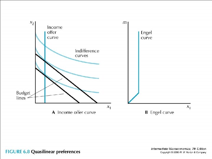
 • A more complicated example • Quasilinear preferences: p 1 = p 2 =1, u(x 1, x 2) = √x 1 + x 2 • MRS 1, 2 = -MU 1 / MU 2 = -p 1/ p 2 • MU 1 = 1/(2 √x 1), MU 2 = 1, MU 1/p 1 = MU 2/p 2 implies x 1 = ¼ is a cutting point
, then becomes vertical •") • IOC: on the x-axis up to (1/4, 0), then becomes vertical • Engel: sloped 1 up to (1/4, 1/4), then becomes vertical • “zero income effect” only after some point
• IOC: on the x-axis up to (1/4, 0), then becomes vertical • Engel: sloped 1 up to (1/4, 1/4), then becomes vertical • “zero income effect” only after some point
 • We now change own price in x 1 (p 1, p 2, m) • ∆x 1/∆p 1 > 0: good 1 is a Giffen good ∆x 1/∆p 1 < 0: good 1 is an ordinary good
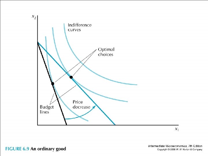
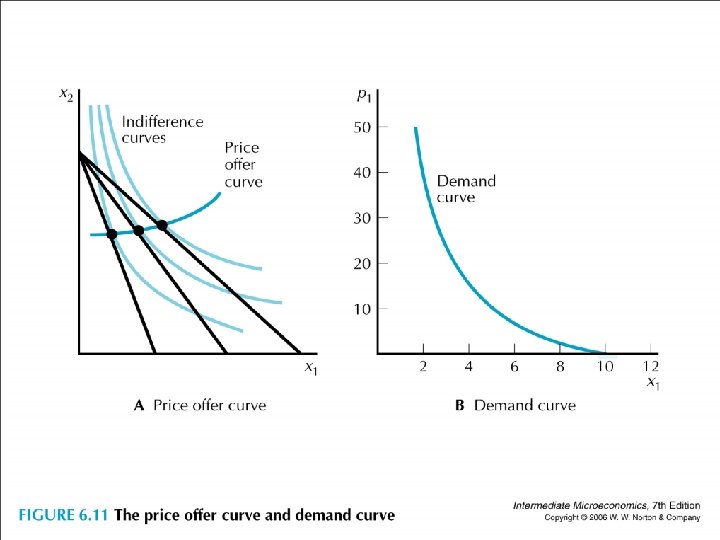
 At x") • Two ways to look at the same thing • (1) At x 1 – x 2 space, connect the demanded bundles as the budget line gets pivoted outward. This curve is called the price offer curve (POC). • (2) At x 1 – p 1 space, connect the optimal x 1 bundles as own price increases while holding income and other price fixed. This curve is called the demand curve.
• Two ways to look at the same thing • (1) At x 1 – x 2 space, connect the demanded bundles as the budget line gets pivoted outward. This curve is called the price offer curve (POC). • (2) At x 1 – p 1 space, connect the optimal x 1 bundles as own price increases while holding income and other price fixed. This curve is called the demand curve.
 • Draw a general preference to illustrate the price offer curve and the demand curve.
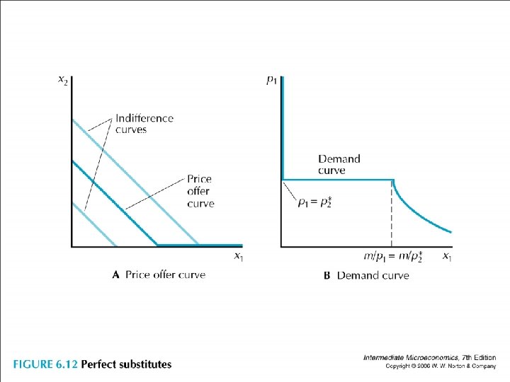
 • Look at specific preferences. • Perfect substitutes: POC p 1 > p 2: x 1 = 0 p 1 = p 2: all budget line p 1 < p 2: x 1 = m/ p 1 draw demand curve
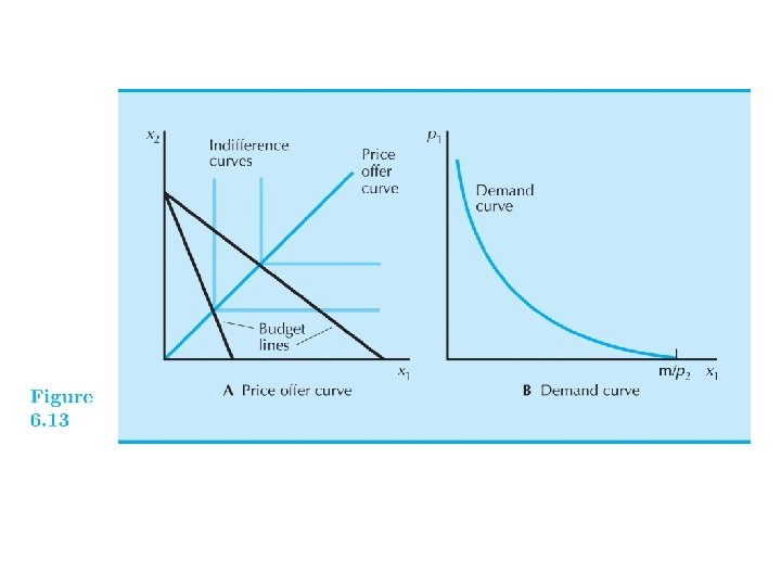
 demand (m/(p 1+p 2))") • Perfect complements: POC (at the corner) demand (m/(p 1+p 2))
• Perfect complements: POC (at the corner) demand (m/(p 1+p 2))
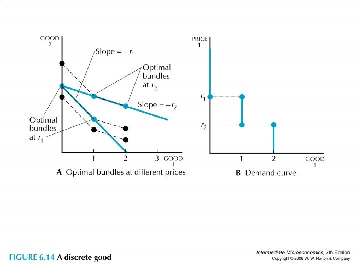
 • A more complicated example • good 1 is in discrete amounts and u(x 1, x 2) = v(x 1) + x 2
 • Suppose m is large enough in the relevant range and let x 2 be the amount of money you can spend on all other goods, then you will start to buy the first unit of good 1 when p 1 has decreased to v(0)+m = v(1)+m-p 1, so p 1 has decreased to v(1) – v(0). • Similarly, you will start buying the second unit of good 1 when p 1 has further decreased to v(1)+m-p 1= v(2)+m-2 p 1, so p 1 has decreased to v(2) – v(1). (draw)
 • Illustrate the demand curve for the quasilinear case
 • We now change other price in x 1 (p 1, p 2, m) • ∆x 1/∆p 2 > 0: good 1 is a substitute for good 2 ∆x 1/∆ p 2 < 0: good 1 is a complement for good 2 (像自己價格的改變)
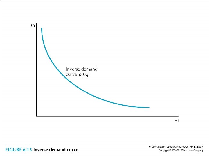
 • We often talk about demand function. • Sometimes it is useful to talk about the inverse demand function x 1 = x 1 (p 1), given p 1, how many x 1 that a consumer wants to buy p 1 = p 1 (x 1), given x 1, what price of p 1 would have to be in order for the consumer to choose that level of consumption
 • Cobb Douglas x 1 = am/ p 1 vs. p 1 = am/ x 1 • Inverse demand has a useful interpretation |MRS 1, 2| = p 1/ p 2 so p 1 = |MRS 1, 2| p 2 suppose good 2 is the money to spend on all other goods, so p 2 = 1 and p 1 = |MRS 1, 2| = ∆$/∆ x 1: how many dollars the individual would be willing to give up to have a little more of 1 (marginal willingness to pay)
 • Demand downward sloping is due to that the marginal willingness to pay decreases as x 1 increases (different from diminishing MRS along an indifference curve as we typically have some surplus when price goes down along the demand curve).
 • Chapter 6 Demand • Key Concept: the demand function x 1 (p 1, p 2, m) • Income m: normal good, inferior good • Own price p 1: Giffen good, ordinary good • Other price p 2: substitute, complement