Chapter 6 Classification and Prediction What is classification

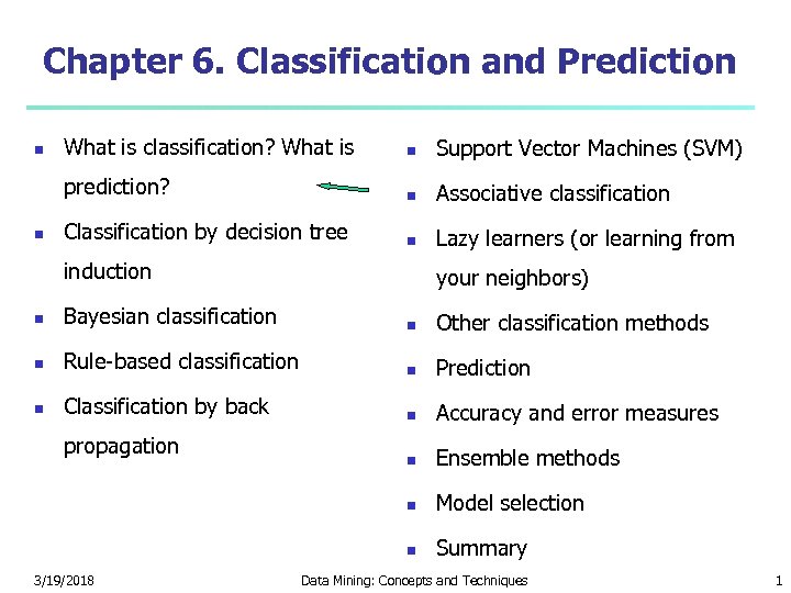Chapter 6. Classification and Prediction What is classification? What is Support Vector Machines (SVM) prediction? Associative classification Classification by decision tree Lazy learners (or learning from induction your neighbors) Bayesian classification Other classification methods Rule-based classification Prediction Classification by back Accuracy and error measures Ensemble methods Model selection Summary propagation 3/19/2018 Data Mining: Concepts and Techniques 1

Classification predicts categorical class labels (discrete or nominal) classifies data (constructs a model) based on the training set and the values (class labels) in a classifying attribute and uses it in classifying new data 3/19/2018 Data Mining: Concepts and Techniques 2

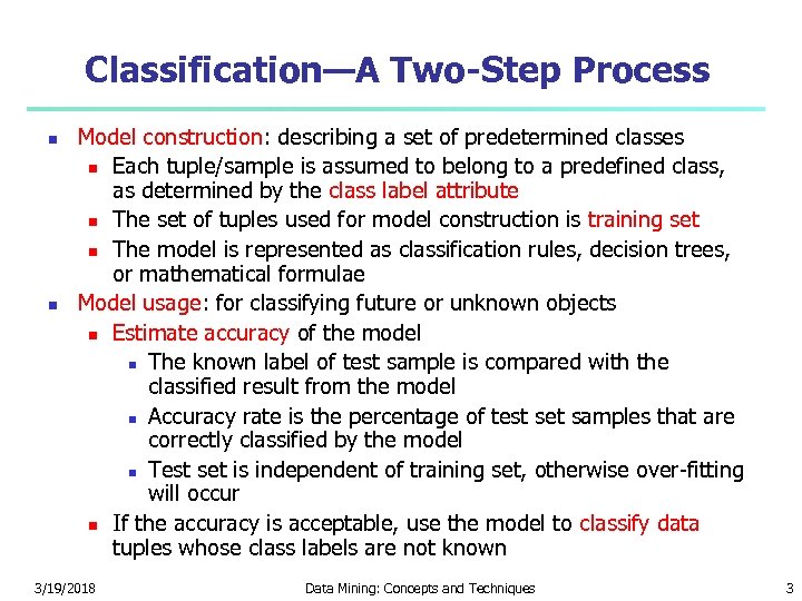Classification—A Two-Step Process Model construction: describing a set of predetermined classes Each tuple/sample is assumed to belong to a predefined class, as determined by the class label attribute The set of tuples used for model construction is training set The model is represented as classification rules, decision trees, or mathematical formulae Model usage: for classifying future or unknown objects Estimate accuracy of the model The known label of test sample is compared with the classified result from the model Accuracy rate is the percentage of test set samples that are correctly classified by the model Test set is independent of training set, otherwise over-fitting will occur If the accuracy is acceptable, use the model to classify data tuples whose class labels are not known 3/19/2018 Data Mining: Concepts and Techniques 3

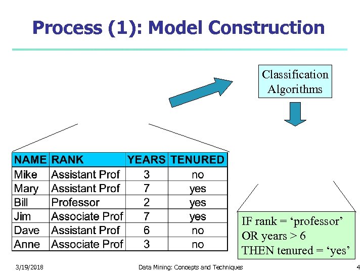Process (1): Model Construction Classification Algorithms IF rank = ‘professor’ OR years > 6 THEN tenured = ‘yes’ 3/19/2018 Data Mining: Concepts and Techniques 4

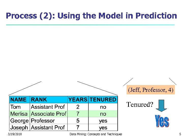Process (2): Using the Model in Prediction (Jeff, Professor, 4) Tenured? 3/19/2018 Data Mining: Concepts and Techniques 5

Supervised vs. Unsupervised Learning Supervised learning (classification) Supervision: The training data (observations, measurements, etc. ) are accompanied by labels indicating the class of the observations New data is classified based on the training set Unsupervised learning (clustering) 3/19/2018 The class labels of training data is unknown Given a set of measurements, observations, etc. with the aim of establishing the existence of classes or clusters in the data Data Mining: Concepts and Techniques 6

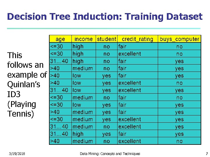Decision Tree Induction: Training Dataset This follows an example of Quinlan’s ID 3 (Playing Tennis) 3/19/2018 Data Mining: Concepts and Techniques 7

Output: A Decision Tree for “buys_computer” 3/19/2018 Data Mining: Concepts and Techniques 8

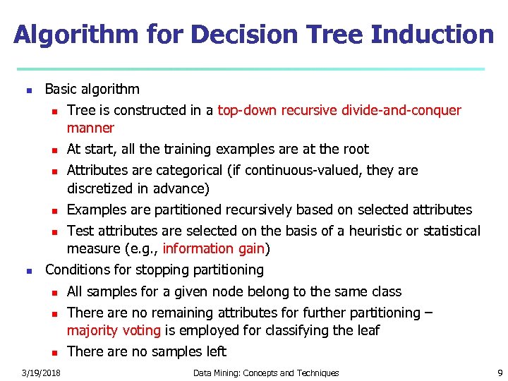Algorithm for Decision Tree Induction Basic algorithm Tree is constructed in a top-down recursive divide-and-conquer manner At start, all the training examples are at the root Attributes are categorical (if continuous-valued, they are discretized in advance) Examples are partitioned recursively based on selected attributes Test attributes are selected on the basis of a heuristic or statistical measure (e. g. , information gain) Conditions for stopping partitioning 3/19/2018 All samples for a given node belong to the same class There are no remaining attributes for further partitioning – majority voting is employed for classifying the leaf There are no samples left Data Mining: Concepts and Techniques 9

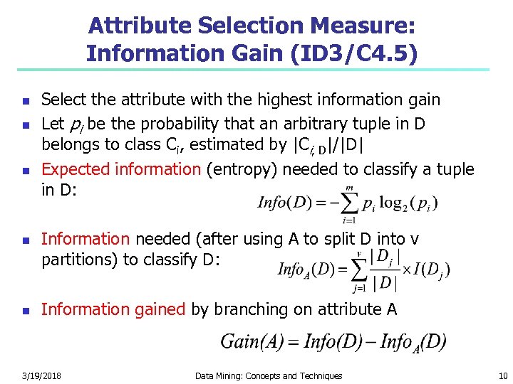Attribute Selection Measure: Information Gain (ID 3/C 4. 5) Select the attribute with the highest information gain Let pi be the probability that an arbitrary tuple in D belongs to class Ci, estimated by |Ci, D|/|D| Expected information (entropy) needed to classify a tuple in D: Information needed (after using A to split D into v partitions) to classify D: Information gained by branching on attribute A 3/19/2018 Data Mining: Concepts and Techniques 10

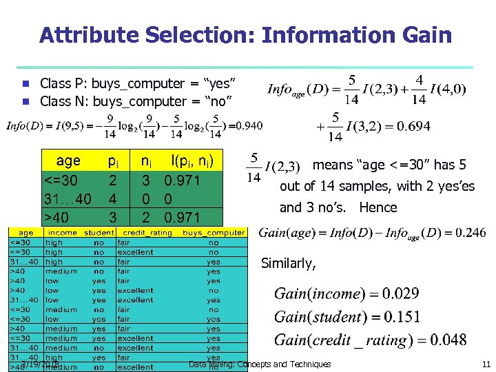Attribute Selection: Information Gain Class P: buys_computer = “yes” Class N: buys_computer = “no” means “age <=30” has 5 out of 14 samples, with 2 yes’es and 3 no’s. Hence Similarly, 3/19/2018 Data Mining: Concepts and Techniques 11

Chapter 6. Classification and Prediction What is classification? What is Support Vector Machines (SVM) prediction? Associative classification Issues regarding classification Lazy learners (or learning from and prediction your neighbors) Classification by decision tree induction Bayesian classification Rule-based classification Classification by back propagation 3/19/2018 Other classification methods Prediction Accuracy and error measures Ensemble methods Model selection Summary Data Mining: Concepts and Techniques 12

Bayesian Classification: Why? A statistical classifier: performs probabilistic prediction, i. e. , predicts class membership probabilities Foundation: Based on Bayes’ Theorem. Performance: A simple Bayesian classifier, naïve Bayesian classifier, has comparable performance with decision tree and selected neural network classifiers Incremental: Each training example can incrementally increase/decrease the probability that a hypothesis is correct — prior knowledge can be combined with observed data Standard: Even when Bayesian methods are computationally intractable, they can provide a standard of optimal decision making against which other methods can be measured 3/19/2018 Data Mining: Concepts and Techniques 13

Bayesian Theorem: Basics Let X be a data sample (training data) Let H be a hypothesis that X belongs to class C Classification is to determine P(H|X), the probability that the hypothesis holds given the observed data sample X P(H) (prior probability), the initial probability E. g. , X will buy computer, regardless of age, income, … P(X): probability that sample data is observed P(X|H) (posteriori probability), the probability of observing the sample X, given that the hypothesis holds 3/19/2018 E. g. , Given that X will buy computer, the probability that X is 31. . 40, and has medium income Data Mining: Concepts and Techniques 14

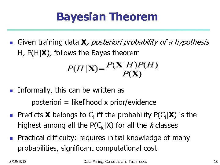Bayesian Theorem Given training data X, posteriori probability of a hypothesis H, P(H|X), follows the Bayes theorem Informally, this can be written as posteriori = likelihood x prior/evidence Predicts X belongs to Ci iff the probability P(Ci|X) is the highest among all the P(Ck|X) for all the k classes Practical difficulty: requires initial knowledge of many probabilities, significant computational cost 3/19/2018 Data Mining: Concepts and Techniques 15

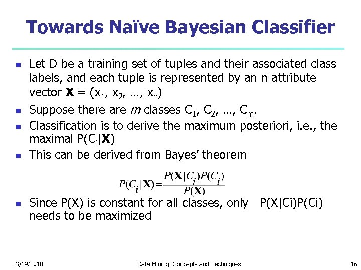Towards Naïve Bayesian Classifier Let D be a training set of tuples and their associated class labels, and each tuple is represented by an n attribute vector X = (x 1, x 2, …, xn) Suppose there are m classes C 1, C 2, …, Cm. Classification is to derive the maximum posteriori, i. e. , the maximal P(Ci|X) This can be derived from Bayes’ theorem Since P(X) is constant for all classes, only P(X|Ci)P(Ci) needs to be maximized 3/19/2018 Data Mining: Concepts and Techniques 16

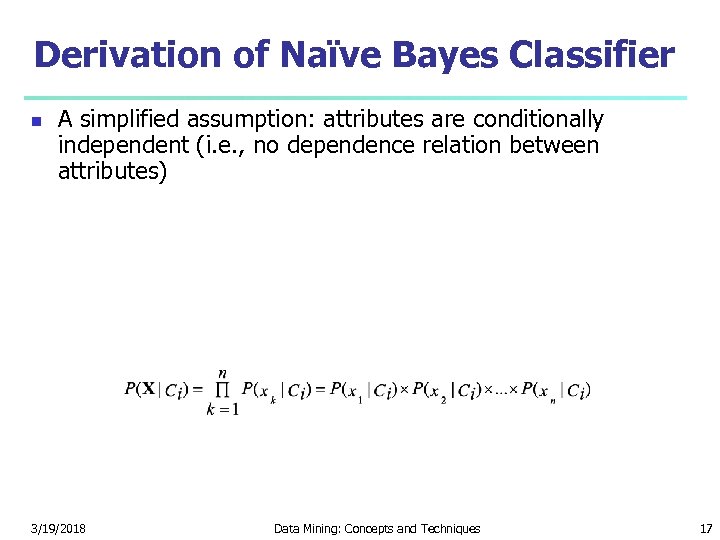Derivation of Naïve Bayes Classifier A simplified assumption: attributes are conditionally independent (i. e. , no dependence relation between attributes) 3/19/2018 Data Mining: Concepts and Techniques 17

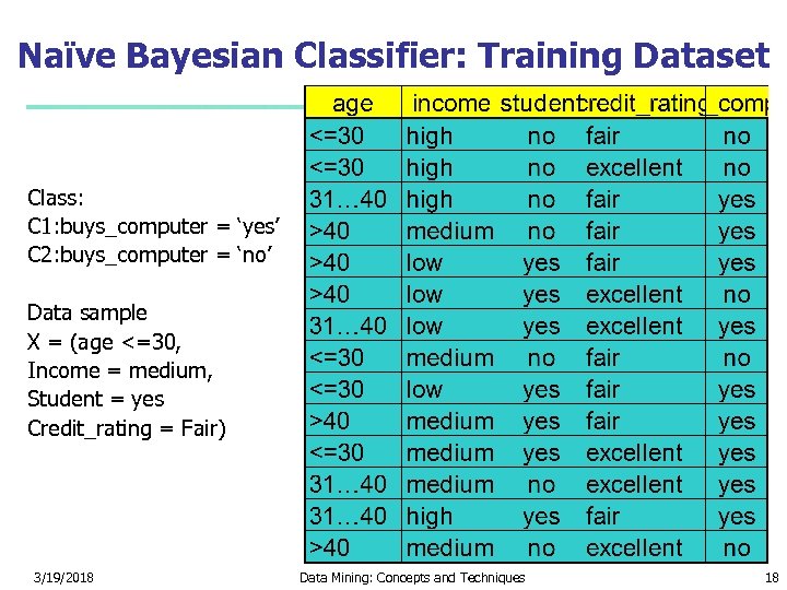Naïve Bayesian Classifier: Training Dataset Class: C 1: buys_computer = ‘yes’ C 2: buys_computer = ‘no’ Data sample X = (age <=30, Income = medium, Student = yes Credit_rating = Fair) 3/19/2018 Data Mining: Concepts and Techniques 18

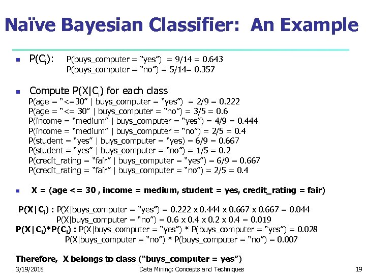Naïve Bayesian Classifier: An Example P(Ci): P(buys_computer = “yes”) = 9/14 = 0. 643 P(buys_computer = “no”) = 5/14= 0. 357 Compute P(X|Ci) for each class P(age = “<=30” | buys_computer = “yes”) = 2/9 = 0. 222 P(age = “<= 30” | buys_computer = “no”) = 3/5 = 0. 6 P(income = “medium” | buys_computer = “yes”) = 4/9 = 0. 444 P(income = “medium” | buys_computer = “no”) = 2/5 = 0. 4 P(student = “yes” | buys_computer = “yes) = 6/9 = 0. 667 P(student = “yes” | buys_computer = “no”) = 1/5 = 0. 2 P(credit_rating = “fair” | buys_computer = “yes”) = 6/9 = 0. 667 P(credit_rating = “fair” | buys_computer = “no”) = 2/5 = 0. 4 X = (age <= 30 , income = medium, student = yes, credit_rating = fair) P(X|Ci) : P(X|buys_computer = “yes”) = 0. 222 x 0. 444 x 0. 667 = 0. 044 P(X|buys_computer = “no”) = 0. 6 x 0. 4 x 0. 2 x 0. 4 = 0. 019 P(X|Ci)*P(Ci) : P(X|buys_computer = “yes”) * P(buys_computer = “yes”) = 0. 028 P(X|buys_computer = “no”) * P(buys_computer = “no”) = 0. 007 Therefore, X belongs to class (“buys_computer = yes”) 3/19/2018 Data Mining: Concepts and Techniques 19

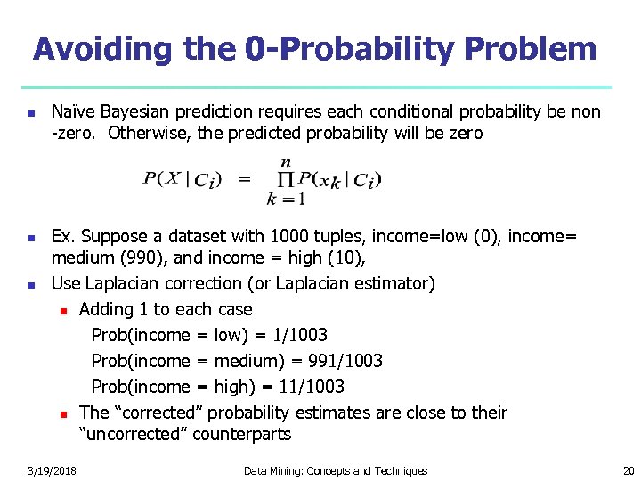Avoiding the 0 -Probability Problem Naïve Bayesian prediction requires each conditional probability be non -zero. Otherwise, the predicted probability will be zero Ex. Suppose a dataset with 1000 tuples, income=low (0), income= medium (990), and income = high (10), Use Laplacian correction (or Laplacian estimator) Adding 1 to each case Prob(income = low) = 1/1003 Prob(income = medium) = 991/1003 Prob(income = high) = 11/1003 The “corrected” probability estimates are close to their “uncorrected” counterparts 3/19/2018 Data Mining: Concepts and Techniques 20

Naïve Bayesian Classifier: Comments Advantages Easy to implement Good results obtained in most of the cases Disadvantages Assumption: class conditional independence, therefore loss of accuracy Practically, dependencies exist among variables E. g. , hospitals: patients: Profile: age, family history, etc. Symptoms: fever, cough etc. , Disease: lung cancer, diabetes, etc. Dependencies among these cannot be modeled by Naïve Bayesian Classifier How to deal with these dependencies? Bayesian Belief Networks 3/19/2018 Data Mining: Concepts and Techniques 21

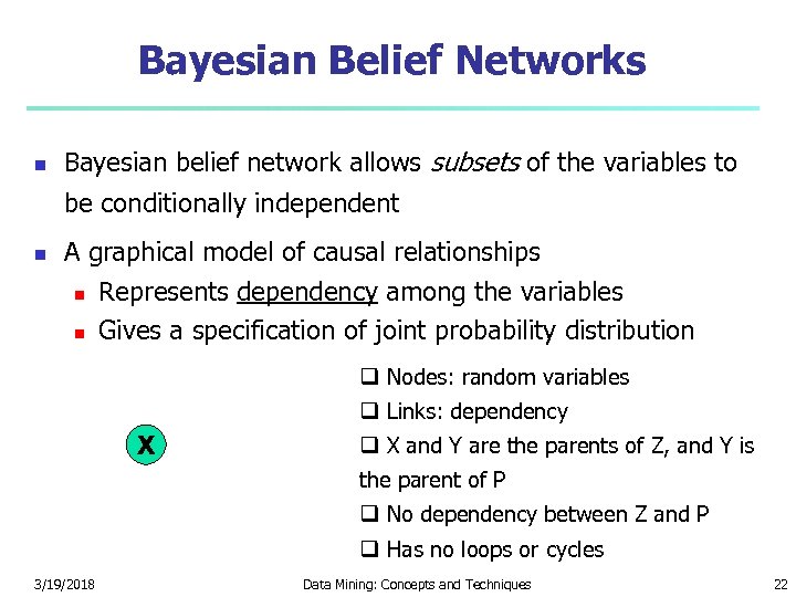Bayesian Belief Networks Bayesian belief network allows subsets of the variables to be conditionally independent A graphical model of causal relationships Represents dependency among the variables Gives a specification of joint probability distribution Nodes: random variables Links: dependency X X and Y are the parents of Z, and Y is the parent of P No dependency between Z and P Has no loops or cycles 3/19/2018 Data Mining: Concepts and Techniques 22

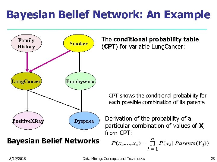Bayesian Belief Network: An Example Family History Lung. Cancer Smoker The conditional probability table (CPT) for variable Lung. Cancer: Emphysema CPT shows the conditional probability for each possible combination of its parents Positive. XRay Dyspnea Bayesian Belief Networks 3/19/2018 Derivation of the probability of a particular combination of values of X, from CPT: Data Mining: Concepts and Techniques 23

Training Bayesian Networks Several scenarios: Given both the network structure and all variables observable: learn only the CPTs Network structure known, some hidden variables: gradient descent (greedy hill-climbing) method, analogous to neural network learning Network structure unknown, all variables observable: search through the model space to reconstruct network topology Unknown structure, all hidden variables: No good algorithms known for this purpose Ref. D. Heckerman: Bayesian networks for data mining 3/19/2018 Data Mining: Concepts and Techniques 24

Chapter 6. Classification and Prediction What is classification? What is Support Vector Machines (SVM) prediction? Associative classification Issues regarding classification Lazy learners (or learning from and prediction your neighbors) Classification by decision tree induction Bayesian classification Rule-based classification Classification by back propagation 3/19/2018 Other classification methods Prediction Accuracy and error measures Ensemble methods Model selection Summary Data Mining: Concepts and Techniques 25

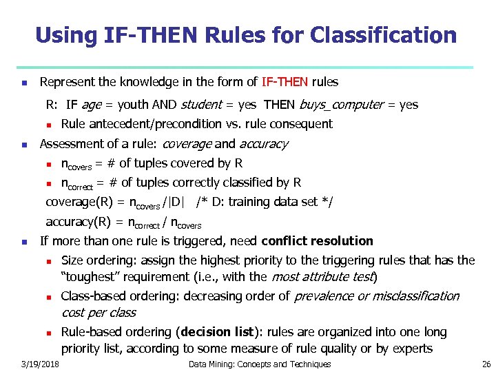Using IF-THEN Rules for Classification Represent the knowledge in the form of IF-THEN rules R: IF age = youth AND student = yes THEN buys_computer = yes Rule antecedent/precondition vs. rule consequent Assessment of a rule: coverage and accuracy ncovers = # of tuples covered by R ncorrect = # of tuples correctly classified by R coverage(R) = ncovers /|D| /* D: training data set */ accuracy(R) = ncorrect / ncovers If more than one rule is triggered, need conflict resolution Size ordering: assign the highest priority to the triggering rules that has the “toughest” requirement (i. e. , with the most attribute test) Class-based ordering: decreasing order of prevalence or misclassification cost per class 3/19/2018 Rule-based ordering (decision list): rules are organized into one long priority list, according to some measure of rule quality or by experts Data Mining: Concepts and Techniques 26

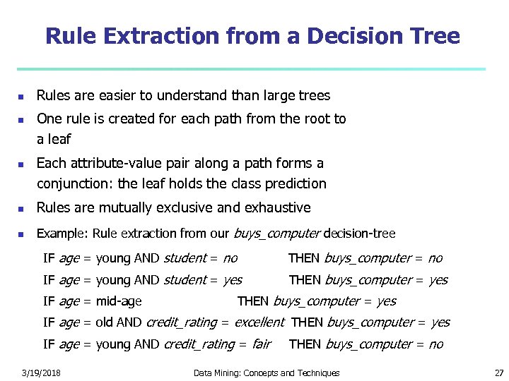Rule Extraction from a Decision Tree Rules are easier to understand than large trees One rule is created for each path from the root to a leaf Each attribute-value pair along a path forms a conjunction: the leaf holds the class prediction Rules are mutually exclusive and exhaustive Example: Rule extraction from our buys_computer decision-tree IF age = young AND student = no THEN buys_computer = no IF age = young AND student = yes THEN buys_computer = yes IF age = mid-age THEN buys_computer = yes IF age = old AND credit_rating = excellent THEN buys_computer = yes IF age = young AND credit_rating = fair THEN buys_computer = no 3/19/2018 Data Mining: Concepts and Techniques 27

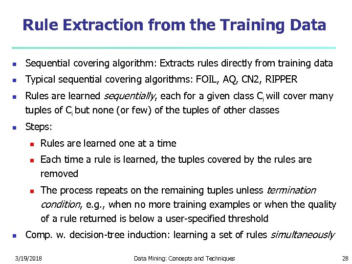Rule Extraction from the Training Data Sequential covering algorithm: Extracts rules directly from training data Typical sequential covering algorithms: FOIL, AQ, CN 2, RIPPER Rules are learned sequentially, each for a given class Ci will cover many tuples of Ci but none (or few) of the tuples of other classes Steps: Rules are learned one at a time Each time a rule is learned, the tuples covered by the rules are removed The process repeats on the remaining tuples unless termination condition, e. g. , when no more training examples or when the quality of a rule returned is below a user-specified threshold Comp. w. decision-tree induction: learning a set of rules simultaneously 3/19/2018 Data Mining: Concepts and Techniques 28

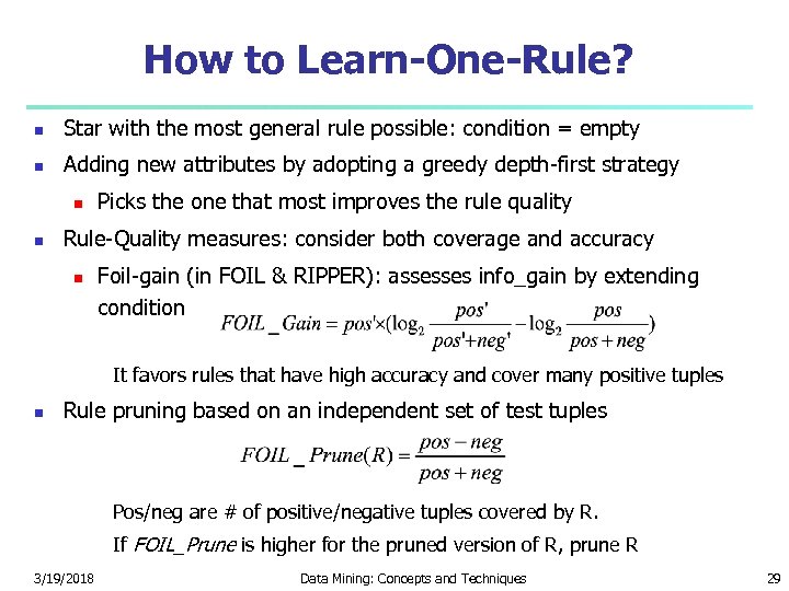How to Learn-One-Rule? Star with the most general rule possible: condition = empty Adding new attributes by adopting a greedy depth-first strategy Picks the one that most improves the rule quality Rule-Quality measures: consider both coverage and accuracy Foil-gain (in FOIL & RIPPER): assesses info_gain by extending condition It favors rules that have high accuracy and cover many positive tuples Rule pruning based on an independent set of test tuples Pos/neg are # of positive/negative tuples covered by R. If FOIL_Prune is higher for the pruned version of R, prune R 3/19/2018 Data Mining: Concepts and Techniques 29

Chapter 6. Classification and Prediction What is classification? What is Support Vector Machines (SVM) prediction? Associative classification Issues regarding classification Lazy learners (or learning from and prediction your neighbors) Classification by decision tree induction Bayesian classification Rule-based classification Classification by back propagation 3/19/2018 Other classification methods Prediction Accuracy and error measures Ensemble methods Model selection Summary Data Mining: Concepts and Techniques 30

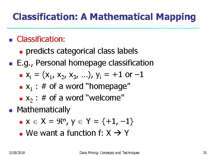Classification: A Mathematical Mapping Classification: predicts categorical class labels E. g. , Personal homepage classification xi = (x 1, x 2, x 3, …), yi = +1 or – 1 x 1 : # of a word “homepage” x 2 : # of a word “welcome” Mathematically n x X = , y Y = {+1, – 1} We want a function f: X Y 3/19/2018 Data Mining: Concepts and Techniques 31

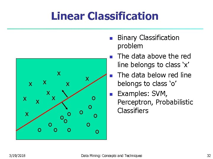Linear Classification x x x 3/19/2018 x x ooo o o x o o o Binary Classification problem The data above the red line belongs to class ‘x’ The data below red line belongs to class ‘o’ Examples: SVM, Perceptron, Probabilistic Classifiers Data Mining: Concepts and Techniques 32

Discriminative Classifiers Advantages prediction accuracy is generally high robust, works when training examples contain errors fast evaluation of the learned target function As compared to Bayesian methods – in general Bayesian networks are normally slow Criticism long training time difficult to understand the learned function (weights) Bayesian networks can be used easily for pattern discovery not easy to incorporate domain knowledge 3/19/2018 Easy in the form of priors on the data or distributions Data Mining: Concepts and Techniques 33

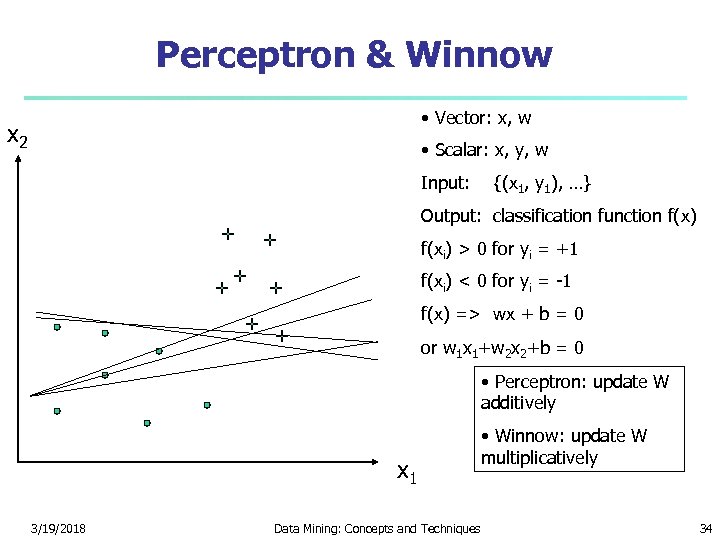Perceptron & Winnow • Vector: x, w x 2 • Scalar: x, y, w Input: {(x 1, y 1), …} Output: classification function f(x) f(xi) > 0 for yi = +1 f(xi) < 0 for yi = -1 f(x) => wx + b = 0 or w 1 x 1+w 2 x 2+b = 0 • Perceptron: update W additively x 1 3/19/2018 Data Mining: Concepts and Techniques • Winnow: update W multiplicatively 34

Classification by Backpropagation Backpropagation: A neural network learning algorithm Started by psychologists and neurobiologists to develop and test computational analogues of neurons A neural network: A set of connected input/output units where each connection has a weight associated with it During the learning phase, the network learns by adjusting the weights so as to be able to predict the correct class label of the input tuples Also referred to as connectionist learning due to the connections between units 3/19/2018 Data Mining: Concepts and Techniques 35

Neural Network as a Classifier Weakness Long training time Require a number of parameters typically best determined empirically, e. g. , the network topology or ``structure. " Poor interpretability: Difficult to interpret the symbolic meaning behind the learned weights and of ``hidden units" in the network Strength 3/19/2018 High tolerance to noisy data Ability to classify untrained patterns Well-suited for continuous-valued inputs and outputs Successful on a wide array of real-world data Algorithms are inherently parallel Techniques have recently been developed for the extraction of rules from trained neural networks Data Mining: Concepts and Techniques 36

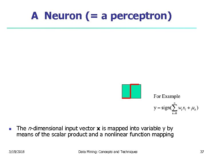A Neuron (= a perceptron) The n-dimensional input vector x is mapped into variable y by means of the scalar product and a nonlinear function mapping 3/19/2018 Data Mining: Concepts and Techniques 37

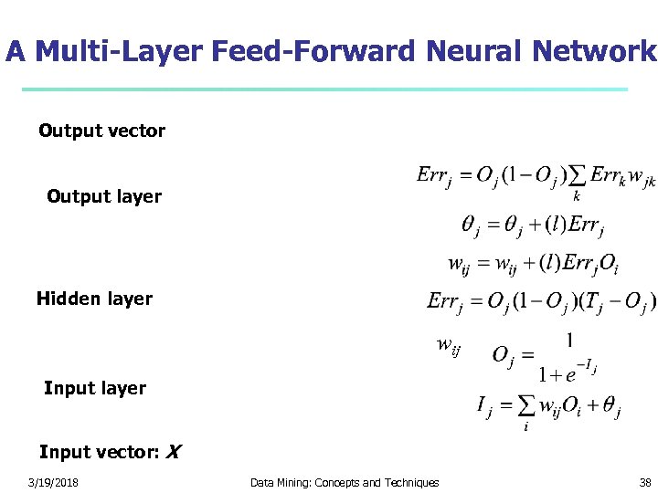A Multi-Layer Feed-Forward Neural Network Output vector Output layer Hidden layer wij Input layer Input vector: X 3/19/2018 Data Mining: Concepts and Techniques 38

How A Multi-Layer Neural Network Works? The inputs to the network correspond to the attributes measured for each training tuple Inputs are fed simultaneously into the units making up the input layer They are then weighted and fed simultaneously to a hidden layer The number of hidden layers is arbitrary, although usually one The weighted outputs of the last hidden layer are input to units making up the output layer, which emits the network's prediction The network is feed-forward in that none of the weights cycles back to an input unit or to an output unit of a previous layer From a statistical point of view, networks perform nonlinear regression: Given enough hidden units and enough training samples, they can closely approximate any function 3/19/2018 Data Mining: Concepts and Techniques 39

Defining a Network Topology First decide the network topology: # of units in the input layer, # of hidden layers (if > 1), # of units in each hidden layer, and # of units in the output layer Normalizing the input values for each attribute measured in the training tuples to [0. 0— 1. 0] One input unit per domain value, each initialized to 0 Output, if for classification and more than two classes, one output unit per class is used Once a network has been trained and its accuracy is unacceptable, repeat the training process with a different network topology or a different set of initial weights 3/19/2018 Data Mining: Concepts and Techniques 40

Backpropagation Iteratively process a set of training tuples & compare the network's prediction with the actual known target value For each training tuple, the weights are modified to minimize the mean squared error between the network's prediction and the actual target value Modifications are made in the “backwards” direction: from the output layer, through each hidden layer down to the first hidden layer, hence “backpropagation” Steps Initialize weights (to small random #s) and biases in the network Propagate the inputs forward (by applying activation function) Backpropagate the error (by updating weights and biases) Terminating condition (when error is very small, etc. ) 3/19/2018 Data Mining: Concepts and Techniques 41

Backpropagation and Interpretability Efficiency of backpropagation: Each epoch (one interation through the training set) takes O(|D| * w), with |D| tuples and w weights, but # of epochs can be exponential to n, the number of inputs, in the worst case Rule extraction from networks: network pruning Simplify the network structure by removing weighted links that have the least effect on the trained network Then perform link, unit, or activation value clustering The set of input and activation values are studied to derive rules describing the relationship between the input and hidden unit layers Sensitivity analysis: assess the impact that a given input variable has on a network output. The knowledge gained from this analysis can be represented in rules 3/19/2018 Data Mining: Concepts and Techniques 42

Chapter 6. Classification and Prediction What is classification? What is Support Vector Machines (SVM) prediction? Associative classification Issues regarding classification Lazy learners (or learning from and prediction your neighbors) Classification by decision tree induction Bayesian classification Rule-based classification Classification by back propagation 3/19/2018 Other classification methods Prediction Accuracy and error measures Ensemble methods Model selection Summary Data Mining: Concepts and Techniques 43

SVM—Support Vector Machines A new classification method for both linear and nonlinear data It uses a nonlinear mapping to transform the original training data into a higher dimension With the new dimension, it searches for the linear optimal separating hyperplane (i. e. , “decision boundary”) With an appropriate nonlinear mapping to a sufficiently high dimension, data from two classes can always be separated by a hyperplane SVM finds this hyperplane using support vectors (“essential” training tuples) and margins (defined by the support vectors) 3/19/2018 Data Mining: Concepts and Techniques 44

SVM—History and Applications Vapnik and colleagues (1992)—groundwork from Vapnik & Chervonenkis’ statistical learning theory in 1960 s Features: training can be slow but accuracy is high owing to their ability to model complex nonlinear decision boundaries (margin maximization) Used both for classification and prediction Applications: handwritten digit recognition, object recognition, speaker identification, benchmarking time-series prediction tests 3/19/2018 Data Mining: Concepts and Techniques 45

SVM—General Philosophy 3/19/2018 Data Mining: Concepts and Techniques 46

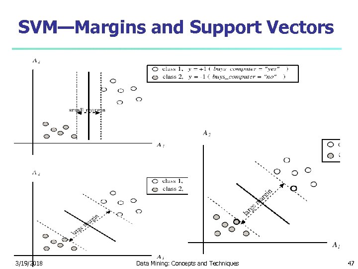SVM—Margins and Support Vectors 3/19/2018 Data Mining: Concepts and Techniques 47

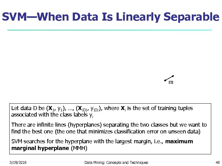SVM—When Data Is Linearly Separable m Let data D be (X 1, y 1), …, (X|D|, y|D|), where Xi is the set of training tuples associated with the class labels yi There are infinite lines (hyperplanes) separating the two classes but we want to find the best one (the one that minimizes classification error on unseen data) SVM searches for the hyperplane with the largest margin, i. e. , maximum marginal hyperplane (MMH) 3/19/2018 Data Mining: Concepts and Techniques 48

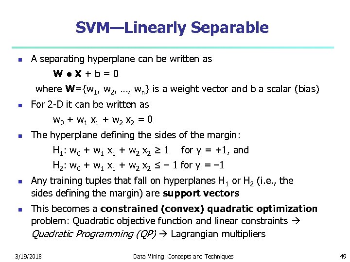SVM—Linearly Separable A separating hyperplane can be written as W ● X + b = 0 where W={w 1, w 2, …, wn} is a weight vector and b a scalar (bias) For 2 -D it can be written as w 0 + w 1 x 1 + w 2 x 2 = 0 The hyperplane defining the sides of the margin: H 1: w 0 + w 1 x 1 + w 2 x 2 ≥ 1 for yi = +1, and H 2: w 0 + w 1 x 1 + w 2 x 2 ≤ – 1 for yi = – 1 Any training tuples that fall on hyperplanes H 1 or H 2 (i. e. , the sides defining the margin) are support vectors This becomes a constrained (convex) quadratic optimization problem: Quadratic objective function and linear constraints Quadratic Programming (QP) Lagrangian multipliers 3/19/2018 Data Mining: Concepts and Techniques 49

Why Is SVM Effective on High Dimensional Data? The complexity of trained classifier is characterized by the # of support vectors rather than the dimensionality of the data The support vectors are the essential or critical training examples — they lie closest to the decision boundary (MMH) If all other training examples are removed and the training is repeated, the same separating hyperplane would be found The number of support vectors found can be used to compute an (upper) bound on the expected error rate of the SVM classifier, which is independent of the data dimensionality Thus, an SVM with a small number of support vectors can have good generalization, even when the dimensionality of the data is high 3/19/2018 Data Mining: Concepts and Techniques 50

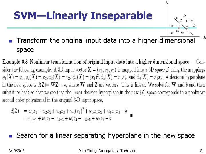SVM—Linearly Inseparable Transform the original input data into a higher dimensional space Search for a linear separating hyperplane in the new space 3/19/2018 Data Mining: Concepts and Techniques 51

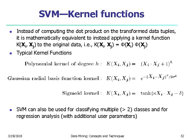SVM—Kernel functions Instead of computing the dot product on the transformed data tuples, it is mathematically equivalent to instead applying a kernel function K(Xi, Xj) to the original data, i. e. , K(Xi, Xj) = Φ(Xi) Φ(Xj) Typical Kernel Functions SVM can also be used for classifying multiple (> 2) classes and for regression analysis (with additional user parameters) 3/19/2018 Data Mining: Concepts and Techniques 52

Scaling SVM by Hierarchical Micro-Clustering SVM is not scalable to the number of data objects in terms of training time and memory usage “Classifying Large Datasets Using SVMs with Hierarchical Clusters Problem” by Hwanjo Yu, Jiong Yang, Jiawei Han, KDD’ 03 CB-SVM (Clustering-Based SVM) Given limited amount of system resources (e. g. , memory), maximize the SVM performance in terms of accuracy and the training speed 3/19/2018 Use micro-clustering to effectively reduce the number of points to be considered At deriving support vectors, de-cluster micro-clusters near “candidate vector” to ensure high classification accuracy Data Mining: Concepts and Techniques 53

CB-SVM: Clustering-Based SVM Training data sets may not even fit in memory Read the data set once (minimizing disk access) Construct a statistical summary of the data (i. e. , hierarchical clusters) given a limited amount of memory The statistical summary maximizes the benefit of learning SVM The summary plays a role in indexing SVMs Essence of Micro-clustering (Hierarchical indexing structure) Use micro-cluster hierarchical indexing structure provide finer samples closer to the boundary and coarser samples farther from the boundary 3/19/2018 Selective de-clustering to ensure high accuracy Data Mining: Concepts and Techniques 54

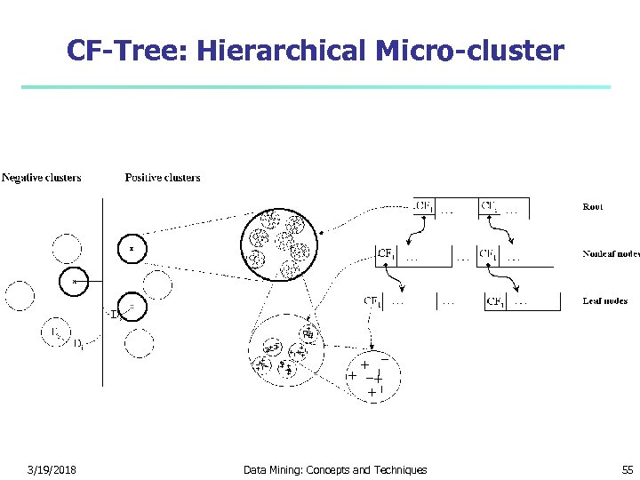CF-Tree: Hierarchical Micro-cluster 3/19/2018 Data Mining: Concepts and Techniques 55

CB-SVM Algorithm: Outline Construct two CF-trees from positive and negative data sets independently Need one scan of the data set Train an SVM from the centroids of the root entries De-cluster the entries near the boundary into the next level The children entries de-clustered from the parent entries are accumulated into the training set with the non-declustered parent entries Train an SVM again from the centroids of the entries in the training set Repeat until nothing is accumulated 3/19/2018 Data Mining: Concepts and Techniques 56

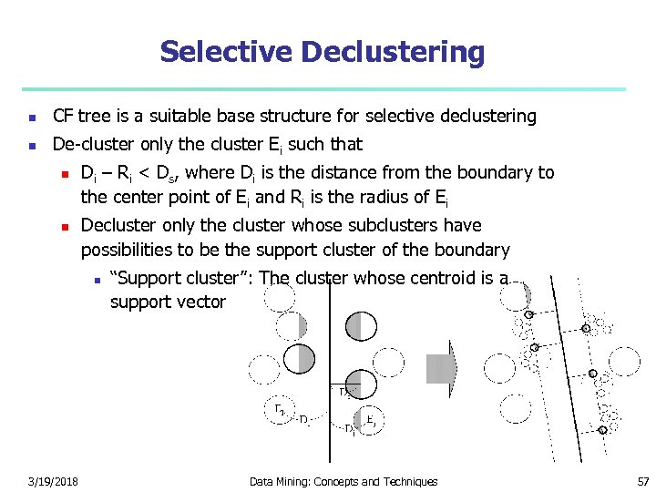Selective Declustering CF tree is a suitable base structure for selective declustering De-cluster only the cluster Ei such that Di – Ri < Ds, where Di is the distance from the boundary to the center point of Ei and Ri is the radius of Ei Decluster only the cluster whose subclusters have possibilities to be the support cluster of the boundary 3/19/2018 “Support cluster”: The cluster whose centroid is a support vector Data Mining: Concepts and Techniques 57

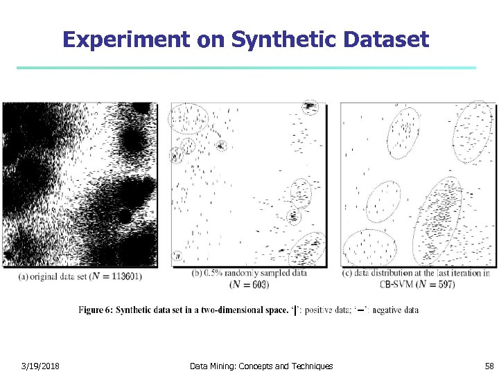Experiment on Synthetic Dataset 3/19/2018 Data Mining: Concepts and Techniques 58

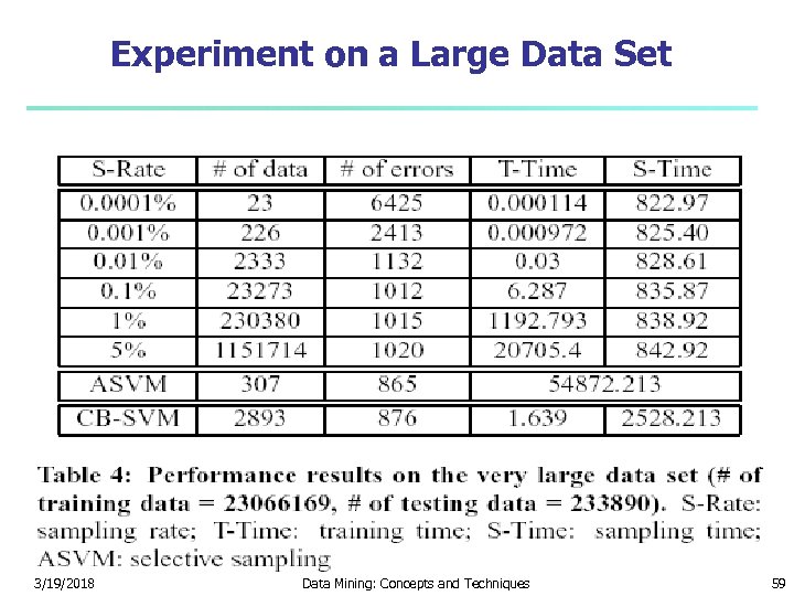Experiment on a Large Data Set 3/19/2018 Data Mining: Concepts and Techniques 59

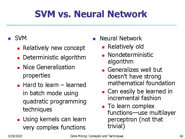SVM vs. Neural Network SVM Relatively new concept Deterministic algorithm 3/19/2018 Nice Generalization properties Hard to learn – learned in batch mode using quadratic programming techniques Using kernels can learn very complex functions Neural Network Relatively old Nondeterministic algorithm Generalizes well but doesn’t have strong mathematical foundation Can easily be learned in incremental fashion To learn complex functions—use multilayer perceptron (not that trivial) Data Mining: Concepts and Techniques 60

SVM Related Links SVM Website http: //www. kernel-machines. org/ Representative implementations LIBSVM: an efficient implementation of SVM, multi-classifications, nu-SVM, one-class SVM, including also various interfaces with java, python, etc. SVM-light: simpler but performance is not better than LIBSVM, support only binary classification and only C language 3/19/2018 SVM-torch: another recent implementation also written in C. Data Mining: Concepts and Techniques 61

SVM—Introduction Literature “Statistical Learning Theory” by Vapnik: extremely hard to understand, containing many errors too. C. J. C. Burges. A Tutorial on Support Vector Machines for Pattern Recognition. Knowledge Discovery and Data Mining, 2(2), 1998. Better than the Vapnik’s book, but still written too hard for introduction, and the examples are so not-intuitive The book “An Introduction to Support Vector Machines” by N. Cristianini and J. Shawe-Taylor Also written hard for introduction, but the explanation about the mercer’s theorem is better than above literatures The neural network book by Haykins 3/19/2018 Contains one nice chapter of SVM introduction Data Mining: Concepts and Techniques 62

Chapter 6. Classification and Prediction What is classification? What is Support Vector Machines (SVM) prediction? Associative classification Issues regarding classification Lazy learners (or learning from and prediction your neighbors) Classification by decision tree induction Bayesian classification Rule-based classification Classification by back propagation 3/19/2018 Other classification methods Prediction Accuracy and error measures Ensemble methods Model selection Summary Data Mining: Concepts and Techniques 63

Associative Classification Associative classification Association rules are generated analyzed for use in classification Search for strong associations between frequent patterns (conjunctions of attribute-value pairs) and class labels Classification: Based on evaluating a set of rules in the form of P 1 ^ p 2 … ^ pl “Aclass = C” (conf, sup) Why effective? It explores highly confident associations among multiple attributes and may overcome some constraints introduced by decision-tree induction, which considers only one attribute at a time In many studies, associative classification has been found to be more accurate than some traditional classification methods, such as C 4. 5 3/19/2018 Data Mining: Concepts and Techniques 64

Typical Associative Classification Methods CBA (Classification By Association: Liu, Hsu & Ma, KDD’ 98) Mine association possible rules in the form of Build classifier: Organize rules according to decreasing precedence based on confidence and then support CMAR (Classification based on Multiple Association Rules: Li, Han, Pei, ICDM’ 01 ) Cond-set (a set of attribute-value pairs) class label Classification: Statistical analysis on multiple rules CPAR (Classification based on Predictive Association Rules: Yin & Han, SDM’ 03 ) Generation of predictive rules (FOIL-like analysis) High efficiency, accuracy similar to CMAR RCBT (Mining top-k covering rule groups for gene expression data, Cong et al. SIGMOD’ 05 ) Explore high-dimensional classification, using top-k rule groups Achieve high classification accuracy and high run-time efficiency 3/19/2018 Data Mining: Concepts and Techniques 65

A Closer Look at CMAR (Classification based on Multiple Association Rules: Li, Han, Pei, ICDM’ 01 ) Efficiency: Uses an enhanced FP-tree that maintains the distribution of class labels among tuples satisfying each frequent itemset Rule pruning whenever a rule is inserted into the tree Given two rules, R 1 and R 2, if the antecedent of R 1 is more general than that of R 2 and conf(R 1) ≥ conf(R 2), then R 2 is pruned Prunes rules for which the rule antecedent and class are not positively correlated, based on a χ2 test of statistical significance Classification based on generated/pruned rules If only one rule satisfies tuple X, assign the class label of the rule If a rule set S satisfies X, CMAR divides S into groups according to class labels 2 uses a weighted χ measure to find the strongest group of rules, based on the statistical correlation of rules within a group assigns X the class label of the strongest group 3/19/2018 Data Mining: Concepts and Techniques 66

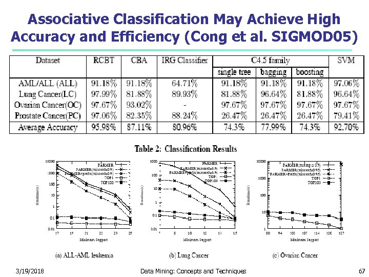Associative Classification May Achieve High Accuracy and Efficiency (Cong et al. SIGMOD 05) 3/19/2018 Data Mining: Concepts and Techniques 67

Chapter 6. Classification and Prediction What is classification? What is Support Vector Machines (SVM) prediction? Associative classification Issues regarding classification Lazy learners (or learning from and prediction your neighbors) Classification by decision tree induction Bayesian classification Rule-based classification Classification by back propagation 3/19/2018 Other classification methods Prediction Accuracy and error measures Ensemble methods Model selection Summary Data Mining: Concepts and Techniques 68

Lazy vs. Eager Learning Lazy vs. eager learning Lazy learning (e. g. , instance-based learning): Simply stores training data (or only minor processing) and waits until it is given a test tuple Eager learning (the above discussed methods): Given a set of training set, constructs a classification model before receiving new (e. g. , test) data to classify Lazy: less time in training but more time in predicting Accuracy Lazy method effectively uses a richer hypothesis space since it uses many local linear functions to form its implicit global approximation to the target function Eager: must commit to a single hypothesis that covers the entire instance space 3/19/2018 Data Mining: Concepts and Techniques 69

Lazy Learner: Instance-Based Methods Instance-based learning: Store training examples and delay the processing (“lazy evaluation”) until a new instance must be classified Typical approaches k-nearest neighbor approach Instances represented as points in a Euclidean space. Locally weighted regression Constructs local approximation Case-based reasoning Uses symbolic representations and knowledgebased inference 3/19/2018 Data Mining: Concepts and Techniques 70

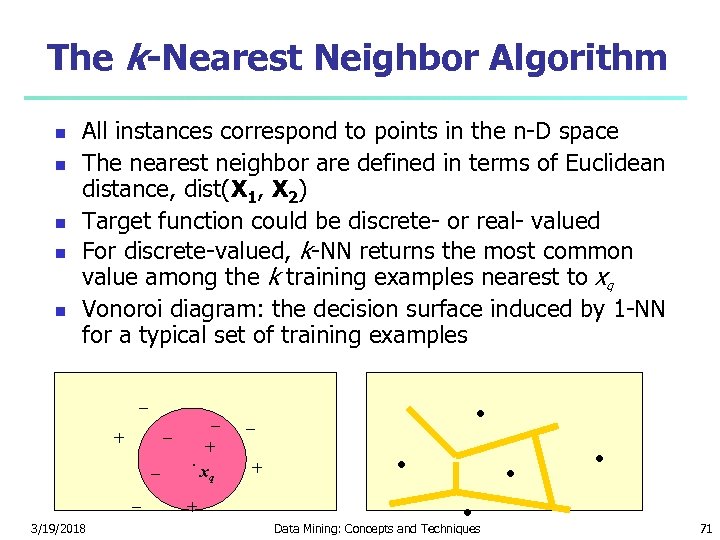The k-Nearest Neighbor Algorithm All instances correspond to points in the n-D space The nearest neighbor are defined in terms of Euclidean distance, dist(X 1, X 2) Target function could be discrete- or real- valued For discrete-valued, k-NN returns the most common value among the k training examples nearest to xq Vonoroi diagram: the decision surface induced by 1 -NN for a typical set of training examples _ _ + _ _ 3/19/2018 _. + + xq . _ + . . Data Mining: Concepts and Techniques . . 71

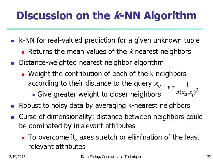Discussion on the k-NN Algorithm k-NN for real-valued prediction for a given unknown tuple Returns the mean values of the k nearest neighbors Distance-weighted nearest neighbor algorithm Weight the contribution of each of the k neighbors according to their distance to the query xq Give greater weight to closer neighbors Robust to noisy data by averaging k-nearest neighbors Curse of dimensionality: distance between neighbors could be dominated by irrelevant attributes 3/19/2018 To overcome it, axes stretch or elimination of the least relevant attributes Data Mining: Concepts and Techniques 72

Case-Based Reasoning (CBR) CBR: Uses a database of problem solutions to solve new problems Store symbolic description (tuples or cases)—not points in a Euclidean space Applications: Customer-service (product-related diagnosis), legal ruling Methodology Instances represented by rich symbolic descriptions (e. g. , function graphs) Search for similar cases, multiple retrieved cases may be combined Tight coupling between case retrieval, knowledge-based reasoning, and problem solving Challenges Find a good similarity metric Indexing based on syntactic similarity measure, and when failure, backtracking, and adapting to additional cases 3/19/2018 Data Mining: Concepts and Techniques 73

Chapter 6. Classification and Prediction What is classification? What is Support Vector Machines (SVM) prediction? Associative classification Issues regarding classification Lazy learners (or learning from and prediction your neighbors) Classification by decision tree induction Bayesian classification Rule-based classification Classification by back propagation 3/19/2018 Other classification methods Prediction Accuracy and error measures Ensemble methods Model selection Summary Data Mining: Concepts and Techniques 74

Genetic Algorithms (GA) Genetic Algorithm: based on an analogy to biological evolution An initial population is created consisting of randomly generated rules E. g. , if A 1 and ¬A 2 then C 2 can be encoded as 100 Each rule is represented by a string of bits If an attribute has k > 2 values, k bits can be used Based on the notion of survival of the fittest, a new population is formed to consist of the fittest rules and their offsprings The fitness of a rule is represented by its classification accuracy on a set of training examples Offsprings are generated by crossover and mutation The process continues until a population P evolves when each rule in P satisfies a prespecified threshold Slow but easily parallelizable 3/19/2018 Data Mining: Concepts and Techniques 75

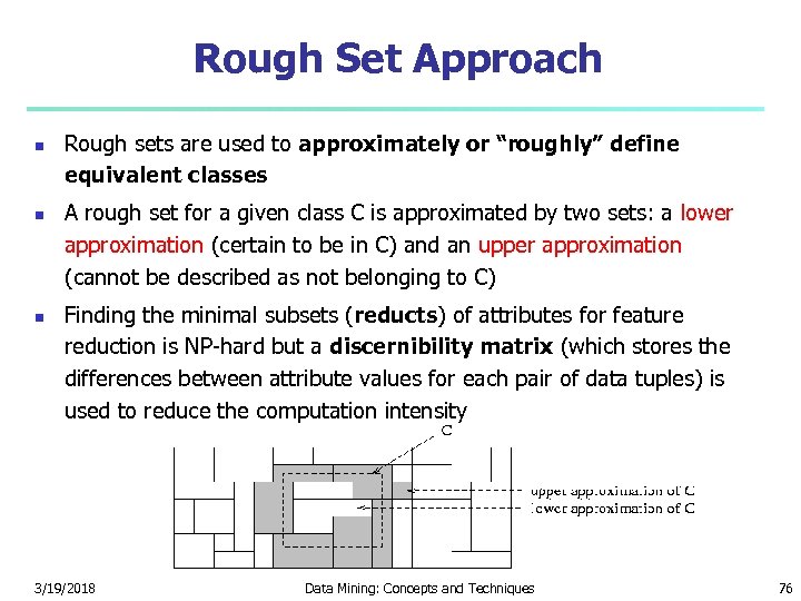Rough Set Approach Rough sets are used to approximately or “roughly” define equivalent classes A rough set for a given class C is approximated by two sets: a lower approximation (certain to be in C) and an upper approximation (cannot be described as not belonging to C) Finding the minimal subsets (reducts) of attributes for feature reduction is NP-hard but a discernibility matrix (which stores the differences between attribute values for each pair of data tuples) is used to reduce the computation intensity 3/19/2018 Data Mining: Concepts and Techniques 76

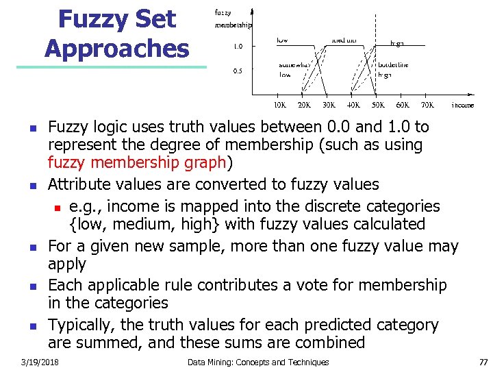Fuzzy Set Approaches Fuzzy logic uses truth values between 0. 0 and 1. 0 to represent the degree of membership (such as using fuzzy membership graph) Attribute values are converted to fuzzy values e. g. , income is mapped into the discrete categories {low, medium, high} with fuzzy values calculated For a given new sample, more than one fuzzy value may apply Each applicable rule contributes a vote for membership in the categories Typically, the truth values for each predicted category are summed, and these sums are combined 3/19/2018 Data Mining: Concepts and Techniques 77

Chapter 6. Classification and Prediction What is classification? What is Support Vector Machines (SVM) prediction? Associative classification Issues regarding classification Lazy learners (or learning from and prediction your neighbors) Classification by decision tree induction Bayesian classification Rule-based classification Classification by back propagation 3/19/2018 Other classification methods Prediction Accuracy and error measures Ensemble methods Model selection Summary Data Mining: Concepts and Techniques 78

What Is Prediction? (Numerical) prediction is similar to classification construct a model use model to predict continuous or ordered value for a given input Prediction is different from classification Classification refers to predict categorical class label Prediction models continuous-valued functions Major method for prediction: regression model the relationship between one or more independent or predictor variables and a dependent or response variable Regression analysis Linear and multiple regression Non-linear regression Other regression methods: generalized linear model, Poisson regression, log-linear models, regression trees 3/19/2018 Data Mining: Concepts and Techniques 79

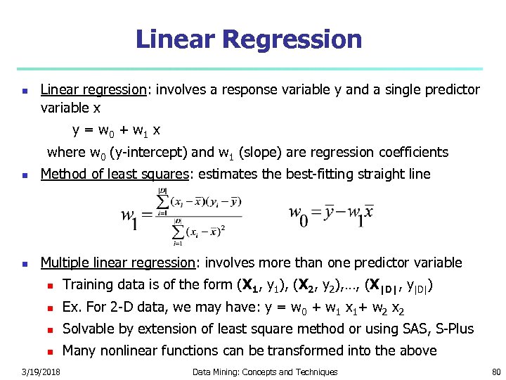Linear Regression Linear regression: involves a response variable y and a single predictor variable x y = w 0 + w 1 x where w 0 (y-intercept) and w 1 (slope) are regression coefficients Method of least squares: estimates the best-fitting straight line Multiple linear regression: involves more than one predictor variable Training data is of the form (X 1, y 1), (X 2, y 2), …, (X|D|, y|D|) Ex. For 2 -D data, we may have: y = w 0 + w 1 x 1+ w 2 x 2 Solvable by extension of least square method or using SAS, S-Plus Many nonlinear functions can be transformed into the above 3/19/2018 Data Mining: Concepts and Techniques 80

Nonlinear Regression Some nonlinear models can be modeled by a polynomial function A polynomial regression model can be transformed into linear regression model. For example, y = w 0 + w 1 x + w 2 x 2 + w 3 x 3 convertible to linear with new variables: x 2 = x 2, x 3= x 3 y = w 0 + w 1 x + w 2 x 2 + w 3 x 3 Other functions, such as power function, can also be transformed to linear model Some models are intractable nonlinear (e. g. , sum of exponential terms) possible to obtain least square estimates through extensive calculation on more complex formulae 3/19/2018 Data Mining: Concepts and Techniques 81

Other Regression-Based Models Generalized linear model: Foundation on which linear regression can be applied to modeling categorical response variables Variance of y is a function of the mean value of y, not a constant Logistic regression: models the prob. of some event occurring as a linear function of a set of predictor variables Poisson regression: models the data that exhibit a Poisson distribution Log-linear models: (for categorical data) Approximate discrete multidimensional prob. distributions Also useful for data compression and smoothing Regression trees and model trees 3/19/2018 Trees to predict continuous values rather than class labels Data Mining: Concepts and Techniques 82

Regression Trees and Model Trees Regression tree: proposed in CART system (Breiman et al. 1984) CART: Classification And Regression Trees Each leaf stores a continuous-valued prediction It is the average value of the predicted attribute for the training tuples that reach the leaf Model tree: proposed by Quinlan (1992) Each leaf holds a regression model—a multivariate linear equation for the predicted attribute A more general case than regression tree Regression and model trees tend to be more accurate than linear regression when the data are not represented well by a simple linear model 3/19/2018 Data Mining: Concepts and Techniques 83

Predictive Modeling in Multidimensional Databases Predictive modeling: Predict data values or construct generalized linear models based on the database data One can only predict value ranges or category distributions Method outline: Minimal generalization Attribute relevance analysis Generalized linear model construction Prediction Determine the major factors which influence the prediction Data relevance analysis: uncertainty measurement, entropy analysis, expert judgement, etc. Multi-level prediction: drill-down and roll-up analysis 3/19/2018 Data Mining: Concepts and Techniques 84

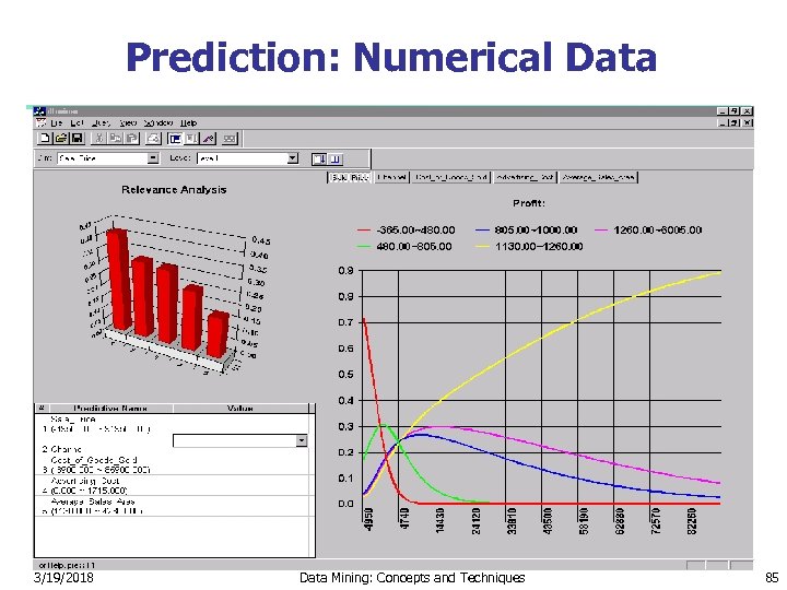Prediction: Numerical Data 3/19/2018 Data Mining: Concepts and Techniques 85

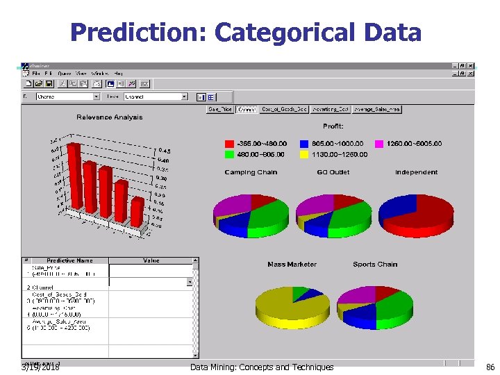Prediction: Categorical Data 3/19/2018 Data Mining: Concepts and Techniques 86

Chapter 6. Classification and Prediction What is classification? What is Support Vector Machines (SVM) prediction? Associative classification Issues regarding classification Lazy learners (or learning from and prediction your neighbors) Classification by decision tree induction Bayesian classification Rule-based classification Classification by back propagation 3/19/2018 Other classification methods Prediction Accuracy and error measures Ensemble methods Model selection Summary Data Mining: Concepts and Techniques 87

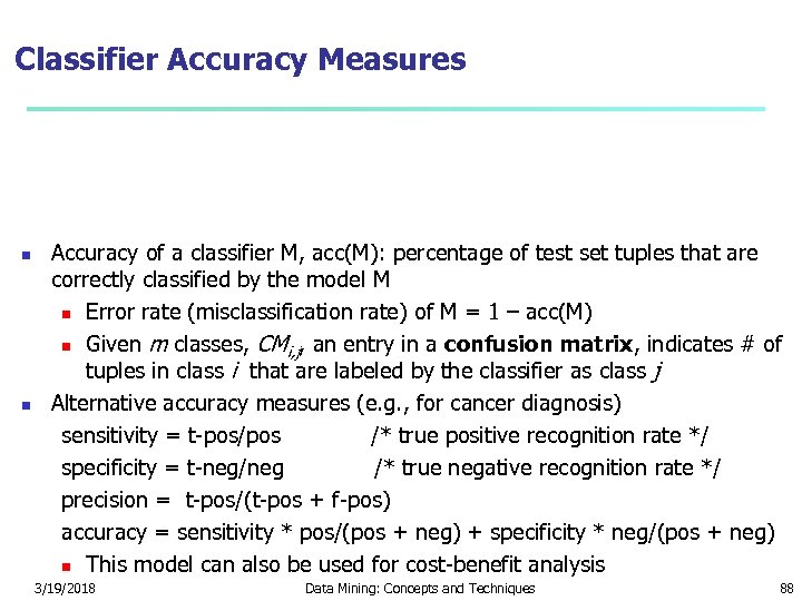Classifier Accuracy Measures Accuracy of a classifier M, acc(M): percentage of test set tuples that are correctly classified by the model M Error rate (misclassification rate) of M = 1 – acc(M) Given m classes, CMi, j, an entry in a confusion matrix, indicates # of tuples in class i that are labeled by the classifier as class j Alternative accuracy measures (e. g. , for cancer diagnosis) sensitivity = t-pos/pos /* true positive recognition rate */ specificity = t-neg/neg /* true negative recognition rate */ precision = t-pos/(t-pos + f-pos) accuracy = sensitivity * pos/(pos + neg) + specificity * neg/(pos + neg) This model can also be used for cost-benefit analysis 3/19/2018 Data Mining: Concepts and Techniques 88

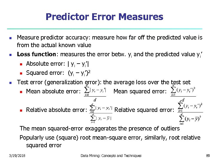Predictor Error Measures Measure predictor accuracy: measure how far off the predicted value is from the actual known value Loss function: measures the error betw. yi and the predicted value yi’ Absolute error: | yi – yi’| Squared error: (yi – yi’)2 Test error (generalization error): the average loss over the test set Mean absolute error: Mean squared error: Relative absolute error: Relative squared error: The mean squared-error exaggerates the presence of outliers Popularly use (square) root mean-square error, similarly, root relative squared error 3/19/2018 Data Mining: Concepts and Techniques 89

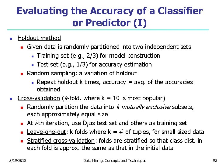Evaluating the Accuracy of a Classifier or Predictor (I) Holdout method Given data is randomly partitioned into two independent sets Training set (e. g. , 2/3) for model construction Test set (e. g. , 1/3) for accuracy estimation Random sampling: a variation of holdout Repeat holdout k times, accuracy = avg. of the accuracies obtained Cross-validation (k-fold, where k = 10 is most popular) Randomly partition the data into k mutually exclusive subsets, each approximately equal size At i-th iteration, use Di as test set and others as training set Leave-one-out: k folds where k = # of tuples, for small sized data Stratified cross-validation: folds are stratified so that class dist. in each fold is approx. the same as that in the initial data 3/19/2018 Data Mining: Concepts and Techniques 90

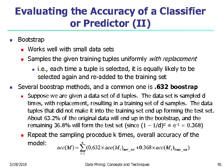Evaluating the Accuracy of a Classifier or Predictor (II) Bootstrap Works well with small data sets Samples the given training tuples uniformly with replacement i. e. , each time a tuple is selected, it is equally likely to be selected again and re-added to the training set Several boostrap methods, and a common one is. 632 boostrap 3/19/2018 Suppose we are given a data set of d tuples. The data set is sampled d times, with replacement, resulting in a training set of d samples. The data tuples that did not make it into the training set end up forming the test set. About 63. 2% of the original data will end up in the bootstrap, and the remaining 36. 8% will form the test set (since (1 – 1/d) d ≈ e-1 = 0. 368) Repeat the sampling procedue k times, overall accuracy of the model: Data Mining: Concepts and Techniques 91

Chapter 6. Classification and Prediction What is classification? What is Support Vector Machines (SVM) prediction? Associative classification Issues regarding classification Lazy learners (or learning from and prediction your neighbors) Classification by decision tree induction Bayesian classification Rule-based classification Classification by back propagation 3/19/2018 Other classification methods Prediction Accuracy and error measures Ensemble methods Model selection Summary Data Mining: Concepts and Techniques 92

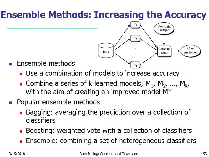Ensemble Methods: Increasing the Accuracy Ensemble methods Use a combination of models to increase accuracy Combine a series of k learned models, M 1, M 2, …, Mk, with the aim of creating an improved model M* Popular ensemble methods Bagging: averaging the prediction over a collection of classifiers Boosting: weighted vote with a collection of classifiers Ensemble: combining a set of heterogeneous classifiers 3/19/2018 Data Mining: Concepts and Techniques 93

Bagging: Boostrap Aggregation Analogy: Diagnosis based on multiple doctors’ majority vote Training Given a set D of d tuples, at each iteration i, a training set Di of d tuples is sampled with replacement from D (i. e. , boostrap) A classifier model Mi is learned for each training set D i Classification: classify an unknown sample X Each classifier Mi returns its class prediction The bagged classifier M* counts the votes and assigns the class with the most votes to X Prediction: can be applied to the prediction of continuous values by taking the average value of each prediction for a given test tuple Accuracy Often significant better than a single classifier derived from D For noise data: not considerably worse, more robust Proved improved accuracy in prediction 3/19/2018 Data Mining: Concepts and Techniques 94

Boosting Analogy: Consult several doctors, based on a combination of weighted diagnoses—weight assigned based on the previous diagnosis accuracy How boosting works? Weights are assigned to each training tuple A series of k classifiers is iteratively learned After a classifier Mi is learned, the weights are updated to allow the subsequent classifier, Mi+1, to pay more attention to the training tuples that were misclassified by Mi The final M* combines the votes of each individual classifier, where the weight of each classifier's vote is a function of its accuracy The boosting algorithm can be extended for the prediction of continuous values Comparing with bagging: boosting tends to achieve greater accuracy, but it also risks overfitting the model to misclassified data 3/19/2018 Data Mining: Concepts and Techniques 95

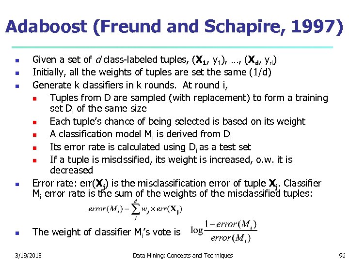Adaboost (Freund and Schapire, 1997) Given a set of d class-labeled tuples, (X 1, y 1), …, (Xd, yd) Initially, all the weights of tuples are set the same (1/d) Generate k classifiers in k rounds. At round i, Tuples from D are sampled (with replacement) to form a training set Di of the same size Each tuple’s chance of being selected is based on its weight A classification model Mi is derived from Di Its error rate is calculated using Di as a test set If a tuple is misclssified, its weight is increased, o. w. it is decreased Error rate: err(Xj) is the misclassification error of tuple Xj. Classifier Mi error rate is the sum of the weights of the misclassified tuples: The weight of classifier Mi’s vote is 3/19/2018 Data Mining: Concepts and Techniques 96

Chapter 6. Classification and Prediction What is classification? What is Support Vector Machines (SVM) prediction? Associative classification Issues regarding classification Lazy learners (or learning from and prediction your neighbors) Classification by decision tree induction Bayesian classification Rule-based classification Classification by back propagation 3/19/2018 Other classification methods Prediction Accuracy and error measures Ensemble methods Model selection Summary Data Mining: Concepts and Techniques 97

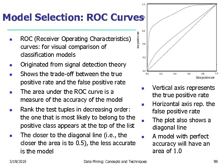Model Selection: ROC Curves ROC (Receiver Operating Characteristics) curves: for visual comparison of classification models Originated from signal detection theory Shows the trade-off between the true positive rate and the false positive rate The area under the ROC curve is a measure of the accuracy of the model Rank the test tuples in decreasing order: the one that is most likely to belong to the positive class appears at the top of the list The closer to the diagonal line (i. e. , the closer the area is to 0. 5), the less accurate is the model 3/19/2018 Data Mining: Concepts and Techniques Vertical axis represents the true positive rate Horizontal axis rep. the false positive rate The plot also shows a diagonal line A model with perfect accuracy will have an area of 1. 0 98

Chapter 6. Classification and Prediction What is classification? What is Support Vector Machines (SVM) prediction? Associative classification Issues regarding classification Lazy learners (or learning from and prediction your neighbors) Classification by decision tree induction Bayesian classification Rule-based classification Classification by back propagation 3/19/2018 Other classification methods Prediction Accuracy and error measures Ensemble methods Model selection Summary Data Mining: Concepts and Techniques 99

Summary (I) Classification and prediction are two forms of data analysis that can be used to extract models describing important data classes or to predict future data trends. Effective and scalable methods have been developed for decision trees induction, Naive Bayesian classification, Bayesian belief network, rule-based classifier, Backpropagation, Support Vector Machine (SVM), associative classification, nearest neighbor classifiers, and case-based reasoning, and other classification methods such as genetic algorithms, rough set and fuzzy set approaches. Linear, nonlinear, and generalized linear models of regression can be used for prediction. Many nonlinear problems can be converted to linear problems by performing transformations on the predictor variables. Regression trees and model trees are also used for prediction. 3/19/2018 Data Mining: Concepts and Techniques 100

Summary (II) Stratified k-fold cross-validation is a recommended method for accuracy estimation. Bagging and boosting can be used to increase overall accuracy by learning and combining a series of individual models. Significance tests and ROC curves are useful for model selection There have been numerous comparisons of the different classification and prediction methods, and the matter remains a research topic No single method has been found to be superior over all others for all data sets Issues such as accuracy, training time, robustness, interpretability, and scalability must be considered and can involve trade-offs, further complicating the quest for an overall superior method 3/19/2018 Data Mining: Concepts and Techniques 101

References (1) C. Apte and S. Weiss. Data mining with decision trees and decision rules. Future Generation Computer Systems, 13, 1997. C. M. Bishop, Neural Networks for Pattern Recognition. Oxford University Press, 1995. L. Breiman, J. Friedman, R. Olshen, and C. Stone. Classification and Regression Trees. Wadsworth International Group, 1984. C. J. C. Burges. A Tutorial on Support Vector Machines for Pattern Recognition. Data Mining and Knowledge Discovery, 2(2): 121 -168, 1998. P. K. Chan and S. J. Stolfo. Learning arbiter and combiner trees from partitioned data for scaling machine learning. KDD'95. W. Cohen. Fast effective rule induction. ICML'95. G. Cong, K. -L. Tan, A. K. H. Tung, and X. Xu. Mining top-k covering rule groups for gene expression data. SIGMOD'05. A. J. Dobson. An Introduction to Generalized Linear Models. Chapman and Hall, 1990. G. Dong and J. Li. Efficient mining of emerging patterns: Discovering trends and differences. KDD'99. 3/19/2018 Data Mining: Concepts and Techniques 102

References (2) R. O. Duda, P. E. Hart, and D. G. Stork. Pattern Classification, 2 ed. John Wiley and Sons, 2001 U. M. Fayyad. Branching on attribute values in decision tree generation. AAAI’ 94. Y. Freund and R. E. Schapire. A decision-theoretic generalization of on-line learning and an application to boosting. J. Computer and System Sciences, 1997. J. Gehrke, R. Ramakrishnan, and V. Ganti. Rainforest: A framework for fast decision tree construction of large datasets. VLDB’ 98. J. Gehrke, V. Gant, R. Ramakrishnan, and W. -Y. Loh, BOAT -- Optimistic Decision Tree Construction. SIGMOD'99. T. Hastie, R. Tibshirani, and J. Friedman. The Elements of Statistical Learning: Data Mining, Inference, and Prediction. Springer-Verlag, 2001. D. Heckerman, D. Geiger, and D. M. Chickering. Learning Bayesian networks: The combination of knowledge and statistical data. Machine Learning, 1995. M. Kamber, L. Winstone, W. Gong, S. Cheng, and J. Han. Generalization and decision tree induction: Efficient classification in data mining. RIDE'97. B. Liu, W. Hsu, and Y. Ma. Integrating Classification and Association Rule. KDD'98. W. Li, J. Han, and J. Pei, CMAR: Accurate and Efficient Classification Based on Multiple Class-Association Rules, ICDM'01. 3/19/2018 Data Mining: Concepts and Techniques 103

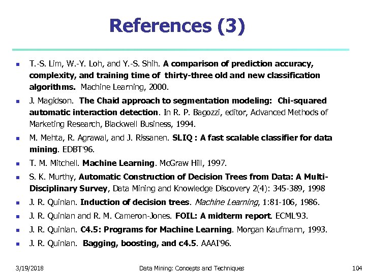References (3) T. -S. Lim, W. -Y. Loh, and Y. -S. Shih. A comparison of prediction accuracy, complexity, and training time of thirty-three old and new classification algorithms. Machine Learning, 2000. J. Magidson. The Chaid approach to segmentation modeling: Chi-squared automatic interaction detection. In R. P. Bagozzi, editor, Advanced Methods of Marketing Research, Blackwell Business, 1994. M. Mehta, R. Agrawal, and J. Rissanen. SLIQ : A fast scalable classifier for data mining. EDBT'96. T. M. Mitchell. Machine Learning. Mc. Graw Hill, 1997. S. K. Murthy, Automatic Construction of Decision Trees from Data: A Multi. Disciplinary Survey, Data Mining and Knowledge Discovery 2(4): 345 -389, 1998 J. R. Quinlan. Induction of decision trees. Machine Learning, 1: 81 -106, 1986. J. R. Quinlan and R. M. Cameron-Jones. FOIL: A midterm report. ECML’ 93. J. R. Quinlan. C 4. 5: Programs for Machine Learning. Morgan Kaufmann, 1993. J. R. Quinlan. Bagging, boosting, and c 4. 5. AAAI'96. 3/19/2018 Data Mining: Concepts and Techniques 104

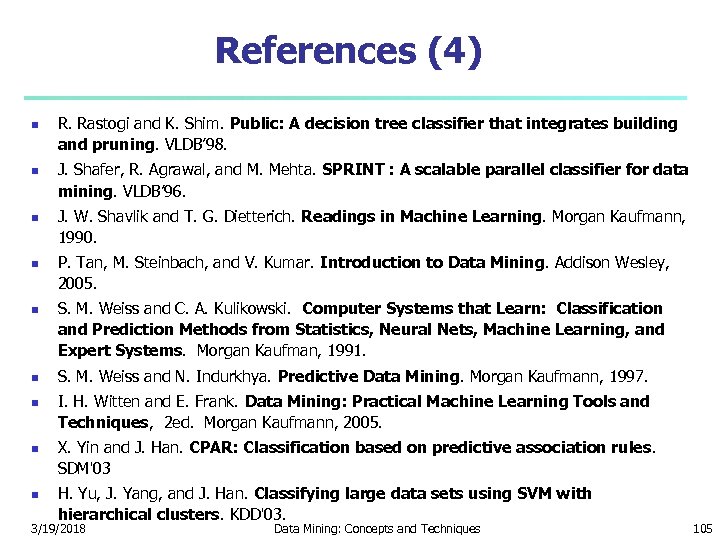References (4) R. Rastogi and K. Shim. Public: A decision tree classifier that integrates building and pruning. VLDB’ 98. J. Shafer, R. Agrawal, and M. Mehta. SPRINT : A scalable parallel classifier for data mining. VLDB’ 96. J. W. Shavlik and T. G. Dietterich. Readings in Machine Learning. Morgan Kaufmann, 1990. P. Tan, M. Steinbach, and V. Kumar. Introduction to Data Mining. Addison Wesley, 2005. S. M. Weiss and C. A. Kulikowski. Computer Systems that Learn: Classification and Prediction Methods from Statistics, Neural Nets, Machine Learning, and Expert Systems. Morgan Kaufman, 1991. S. M. Weiss and N. Indurkhya. Predictive Data Mining. Morgan Kaufmann, 1997. I. H. Witten and E. Frank. Data Mining: Practical Machine Learning Tools and Techniques, 2 ed. Morgan Kaufmann, 2005. X. Yin and J. Han. CPAR: Classification based on predictive association rules. SDM'03 H. Yu, J. Yang, and J. Han. Classifying large data sets using SVM with hierarchical clusters. KDD'03. 3/19/2018 Data Mining: Concepts and Techniques 105

3/19/2018 Data Mining: Concepts and Techniques 106