Chapter 6 Classification and Prediction n What is

Chapter 6. Classification and Prediction n What is classification? What is n Support Vector Machines (SVM) prediction? n n Associative classification Issues regarding classification n Lazy learners (or learning from and prediction n your neighbors) Classification by decision tree induction n Bayesian classification n Rule-based classification n Classification by back propagation 15 March 2018 n Other classification methods n Prediction n Accuracy and error measures n Ensemble methods n Model selection n Summary Data Mining: Concepts and Techniques 1

Classification vs. Prediction n n Classification n predicts categorical class labels (discrete or nominal) n classifies data (constructs a model) based on the training set and the values (class labels) in a classifying attribute and uses it in classifying new data Prediction n models continuous-valued functions, i. e. , predicts unknown or missing values 15 March 2018 Data Mining: Concepts and Techniques 2

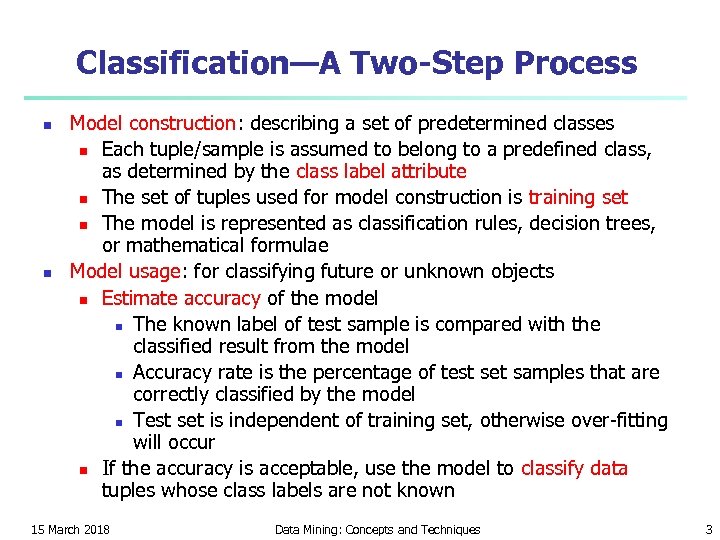Classification—A Two-Step Process n n Model construction: describing a set of predetermined classes n Each tuple/sample is assumed to belong to a predefined class, as determined by the class label attribute n The set of tuples used for model construction is training set n The model is represented as classification rules, decision trees, or mathematical formulae Model usage: for classifying future or unknown objects n Estimate accuracy of the model n The known label of test sample is compared with the classified result from the model n Accuracy rate is the percentage of test set samples that are correctly classified by the model n Test set is independent of training set, otherwise over-fitting will occur n If the accuracy is acceptable, use the model to classify data tuples whose class labels are not known 15 March 2018 Data Mining: Concepts and Techniques 3

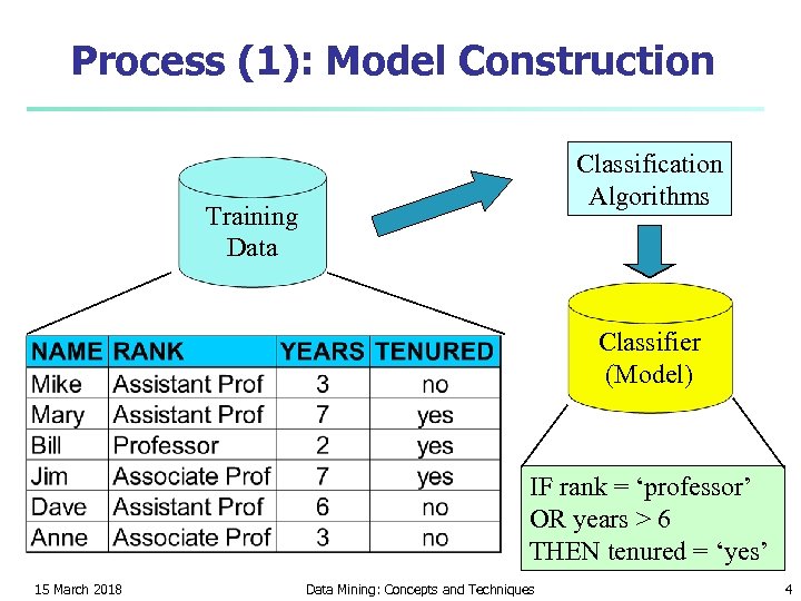Process (1): Model Construction Classification Algorithms Training Data Classifier (Model) IF rank = ‘professor’ OR years > 6 THEN tenured = ‘yes’ 15 March 2018 Data Mining: Concepts and Techniques 4

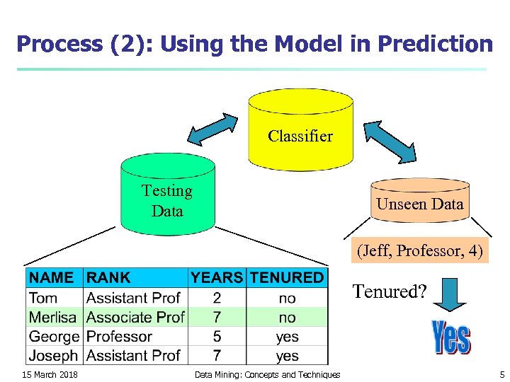Process (2): Using the Model in Prediction Classifier Testing Data Unseen Data (Jeff, Professor, 4) Tenured? 15 March 2018 Data Mining: Concepts and Techniques 5

Supervised vs. Unsupervised Learning n Supervised learning (classification) n n n Supervision: The training data (observations, measurements, etc. ) are accompanied by labels indicating the class of the observations New data is classified based on the training set Unsupervised learning (clustering) n n 15 March 2018 The class labels of training data is unknown Given a set of measurements, observations, etc. with the aim of establishing the existence of classes or clusters in the data Data Mining: Concepts and Techniques 6

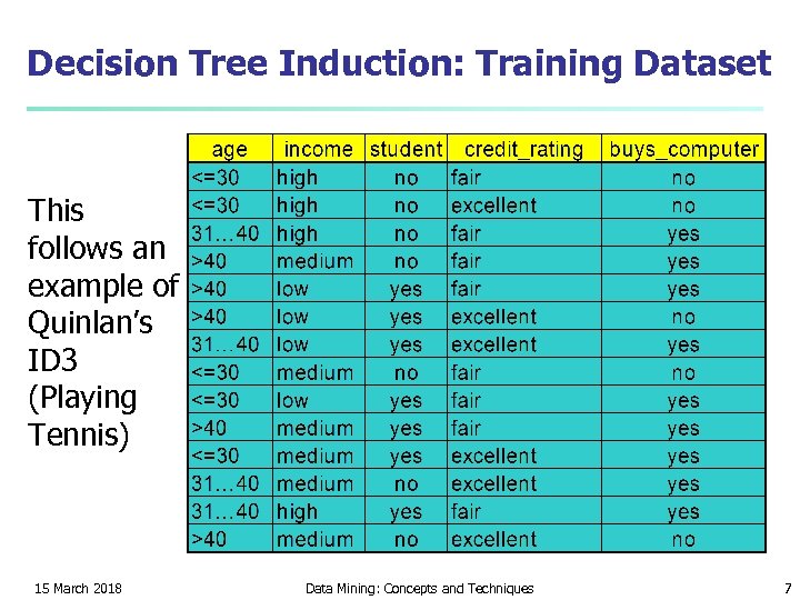Decision Tree Induction: Training Dataset This follows an example of Quinlan’s ID 3 (Playing Tennis) 15 March 2018 Data Mining: Concepts and Techniques 7

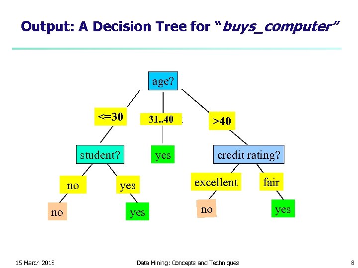Output: A Decision Tree for “buys_computer” age? <=30 31. . 40 overcast student? no no 15 March 2018 >40 credit rating? yes excellent yes no Data Mining: Concepts and Techniques fair yes 8

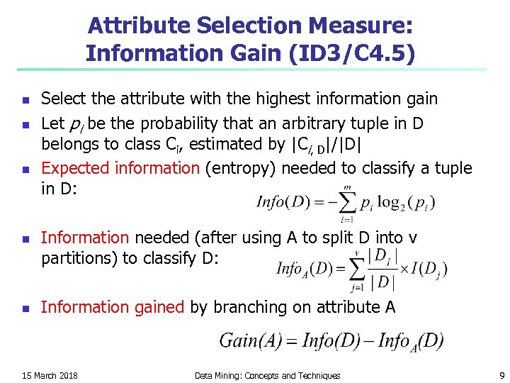Attribute Selection Measure: Information Gain (ID 3/C 4. 5) n n n Select the attribute with the highest information gain Let pi be the probability that an arbitrary tuple in D belongs to class Ci, estimated by |Ci, D|/|D| Expected information (entropy) needed to classify a tuple in D: Information needed (after using A to split D into v partitions) to classify D: Information gained by branching on attribute A 15 March 2018 Data Mining: Concepts and Techniques 9

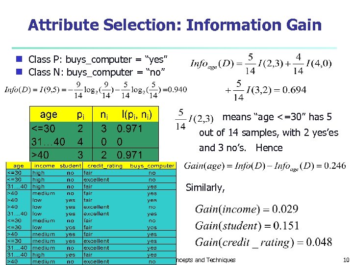Attribute Selection: Information Gain Class P: buys_computer = “yes” g Class N: buys_computer = “no” g means “age <=30” has 5 out of 14 samples, with 2 yes’es and 3 no’s. Hence Similarly, 15 March 2018 Data Mining: Concepts and Techniques 10

Computing Information-Gain for Continuous-Value Attributes n Let attribute A be a continuous-valued attribute n Must determine the best split point for A n n Sort the value A in increasing order Typically, the midpoint between each pair of adjacent values is considered as a possible split point n n n (ai+ai+1)/2 is the midpoint between the values of ai and ai+1 The point with the minimum expected information requirement for A is selected as the split-point for A Split: n D 1 is the set of tuples in D satisfying A ≤ split-point, and D 2 is the set of tuples in D satisfying A > split-point 15 March 2018 Data Mining: Concepts and Techniques 11

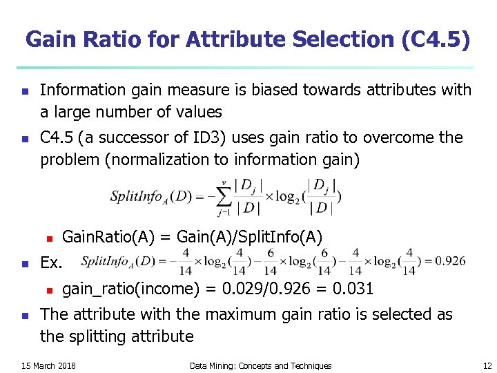Gain Ratio for Attribute Selection (C 4. 5) n n Information gain measure is biased towards attributes with a large number of values C 4. 5 (a successor of ID 3) uses gain ratio to overcome the problem (normalization to information gain) n n Ex. n n Gain. Ratio(A) = Gain(A)/Split. Info(A) gain_ratio(income) = 0. 029/0. 926 = 0. 031 The attribute with the maximum gain ratio is selected as the splitting attribute 15 March 2018 Data Mining: Concepts and Techniques 12

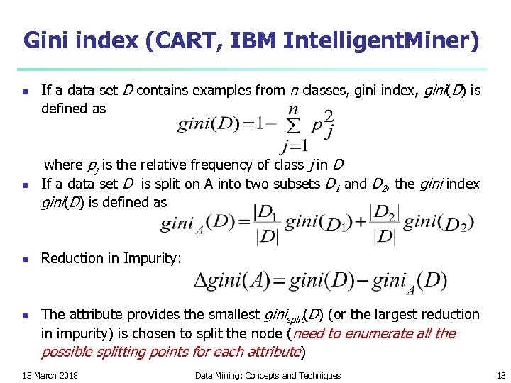Gini index (CART, IBM Intelligent. Miner) n If a data set D contains examples from n classes, gini index, gini(D) is defined as n where pj is the relative frequency of class j in D If a data set D is split on A into two subsets D 1 and D 2, the gini index gini(D) is defined as n Reduction in Impurity: n The attribute provides the smallest ginisplit(D) (or the largest reduction in impurity) is chosen to split the node (need to enumerate all the possible splitting points for each attribute) 15 March 2018 Data Mining: Concepts and Techniques 13

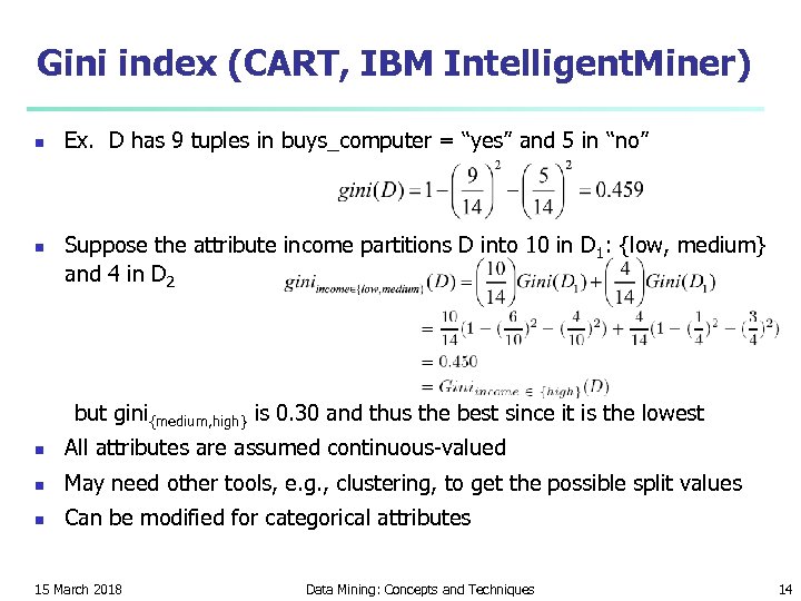Gini index (CART, IBM Intelligent. Miner) n n Ex. D has 9 tuples in buys_computer = “yes” and 5 in “no” Suppose the attribute income partitions D into 10 in D 1: {low, medium} and 4 in D 2 but gini{medium, high} is 0. 30 and thus the best since it is the lowest n All attributes are assumed continuous-valued n May need other tools, e. g. , clustering, to get the possible split values n Can be modified for categorical attributes 15 March 2018 Data Mining: Concepts and Techniques 14

Classification in Large Databases n n n Classification—a classical problem extensively studied by statisticians and machine learning researchers Scalability: Classifying data sets with millions of examples and hundreds of attributes with reasonable speed Why decision tree induction in data mining? n relatively faster learning speed (than other classification methods) n convertible to simple and easy to understand classification rules n can use SQL queries for accessing databases n comparable classification accuracy with other methods 15 March 2018 Data Mining: Concepts and Techniques 15

BOAT (Bootstrapped Optimistic Algorithm for Tree Construction) n Use a statistical technique called bootstrapping to create several smaller samples (subsets), each fits in memory n Each subset is used to create a tree, resulting in several trees n These trees are examined and used to construct a new tree T’ n It turns out that T’ is very close to the tree that would be generated using the whole data set together n Adv: requires only two scans of DB, an incremental alg. 15 March 2018 Data Mining: Concepts and Techniques 16

Bayesian Classification: Why? n n n A statistical classifier: performs probabilistic prediction, i. e. , predicts class membership probabilities Foundation: Based on Bayes’ Theorem. Performance: A simple Bayesian classifier, naïve Bayesian classifier, has comparable performance with decision tree and selected neural network classifiers Incremental: Each training example can incrementally increase/decrease the probability that a hypothesis is correct — prior knowledge can be combined with observed data Standard: Even when Bayesian methods are computationally intractable, they can provide a standard of optimal decision making against which other methods can be measured 15 March 2018 Data Mining: Concepts and Techniques 17

Bayesian Theorem: Basics n Let X be a data sample (“evidence”): class label is unknown n Let H be a hypothesis that X belongs to class C n n Classification is to determine P(H|X), the probability that the hypothesis holds given the observed data sample X P(H) (prior probability), the initial probability n n n E. g. , X will buy computer, regardless of age, income, … P(X): probability that sample data is observed P(X|H) (posteriori probability), the probability of observing the sample X, given that the hypothesis holds n E. g. , Given that X will buy computer, the prob. that X is 31. . 40, medium income 15 March 2018 Data Mining: Concepts and Techniques 18

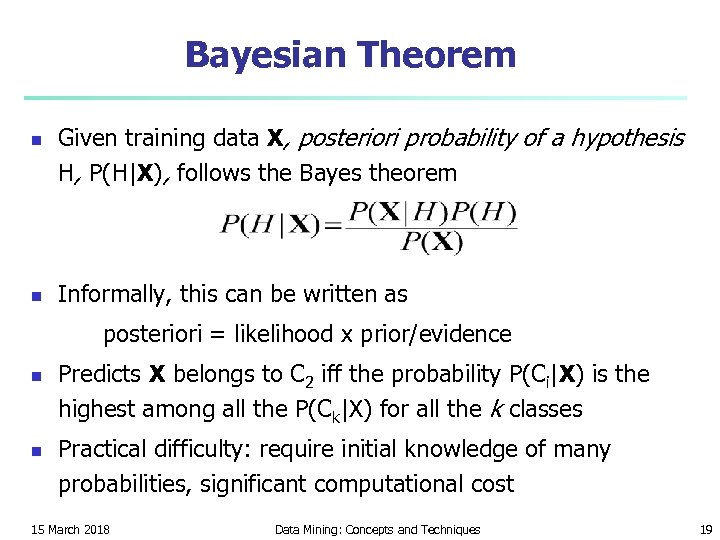Bayesian Theorem n n Given training data X, posteriori probability of a hypothesis H, P(H|X), follows the Bayes theorem Informally, this can be written as posteriori = likelihood x prior/evidence n n Predicts X belongs to C 2 iff the probability P(Ci|X) is the highest among all the P(Ck|X) for all the k classes Practical difficulty: require initial knowledge of many probabilities, significant computational cost 15 March 2018 Data Mining: Concepts and Techniques 19

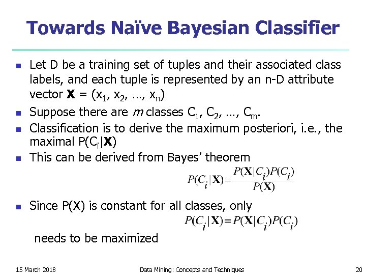Towards Naïve Bayesian Classifier n Let D be a training set of tuples and their associated class labels, and each tuple is represented by an n-D attribute vector X = (x 1, x 2, …, xn) Suppose there are m classes C 1, C 2, …, Cm. Classification is to derive the maximum posteriori, i. e. , the maximal P(Ci|X) This can be derived from Bayes’ theorem n Since P(X) is constant for all classes, only n needs to be maximized 15 March 2018 Data Mining: Concepts and Techniques 20

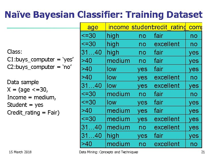Naïve Bayesian Classifier: Training Dataset Class: C 1: buys_computer = ‘yes’ C 2: buys_computer = ‘no’ Data sample X = (age <=30, Income = medium, Student = yes Credit_rating = Fair) 15 March 2018 Data Mining: Concepts and Techniques 21

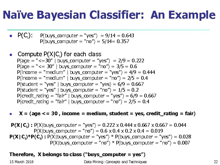Naïve Bayesian Classifier: An Example n P(Ci): n Compute P(X|Ci) for each class P(buys_computer = “yes”) = 9/14 = 0. 643 P(buys_computer = “no”) = 5/14= 0. 357 P(age = “<=30” | buys_computer = “yes”) = 2/9 = 0. 222 P(age = “<= 30” | buys_computer = “no”) = 3/5 = 0. 6 P(income = “medium” | buys_computer = “yes”) = 4/9 = 0. 444 P(income = “medium” | buys_computer = “no”) = 2/5 = 0. 4 P(student = “yes” | buys_computer = “yes) = 6/9 = 0. 667 P(student = “yes” | buys_computer = “no”) = 1/5 = 0. 2 P(credit_rating = “fair” | buys_computer = “yes”) = 6/9 = 0. 667 P(credit_rating = “fair” | buys_computer = “no”) = 2/5 = 0. 4 n X = (age <= 30 , income = medium, student = yes, credit_rating = fair) P(X|Ci) : P(X|buys_computer = “yes”) = 0. 222 x 0. 444 x 0. 667 = 0. 044 P(X|buys_computer = “no”) = 0. 6 x 0. 4 x 0. 2 x 0. 4 = 0. 019 P(X|Ci)*P(Ci) : P(X|buys_computer = “yes”) * P(buys_computer = “yes”) = 0. 028 P(X|buys_computer = “no”) * P(buys_computer = “no”) = 0. 007 Therefore, X belongs to class (“buys_computer = yes”) 15 March 2018 Data Mining: Concepts and Techniques 22

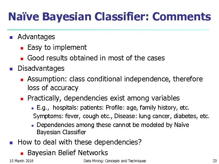Naïve Bayesian Classifier: Comments n n Advantages n Easy to implement n Good results obtained in most of the cases Disadvantages n Assumption: class conditional independence, therefore loss of accuracy n Practically, dependencies exist among variables E. g. , hospitals: patients: Profile: age, family history, etc. Symptoms: fever, cough etc. , Disease: lung cancer, diabetes, etc. n Dependencies among these cannot be modeled by Naïve Bayesian Classifier n n How to deal with these dependencies? n Bayesian Belief Networks 15 March 2018 Data Mining: Concepts and Techniques 23

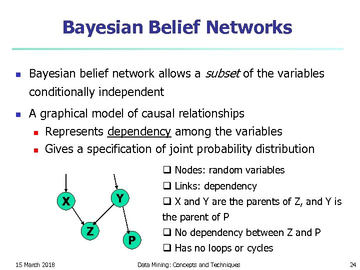Bayesian Belief Networks n Bayesian belief network allows a subset of the variables conditionally independent n A graphical model of causal relationships n n Represents dependency among the variables Gives a specification of joint probability distribution q Nodes: random variables q Links: dependency Y X q X and Y are the parents of Z, and Y is the parent of P Z 15 March 2018 P q No dependency between Z and P q Has no loops or cycles Data Mining: Concepts and Techniques 24

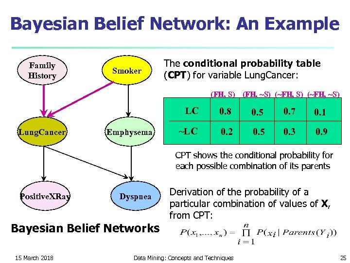Bayesian Belief Network: An Example Family History Smoker The conditional probability table (CPT) for variable Lung. Cancer: (FH, S) (FH, ~S) (~FH, ~S) LC Lung. Cancer Emphysema 0. 8 0. 5 0. 7 0. 1 ~LC 0. 2 0. 5 0. 3 0. 9 CPT shows the conditional probability for each possible combination of its parents Positive. XRay Dyspnea Bayesian Belief Networks 15 March 2018 Derivation of the probability of a particular combination of values of X, from CPT: Data Mining: Concepts and Techniques 25

Classification by Backpropagation n n Backpropagation: A neural network learning algorithm Started by psychologists and neurobiologists to develop and test computational analogues of neurons A neural network: A set of connected input/output units where each connection has a weight associated with it During the learning phase, the network learns by adjusting the weights so as to be able to predict the correct class label of the input tuples Also referred to as connectionist learning due to the connections between units 15 March 2018 Data Mining: Concepts and Techniques 26

Neural Network as a Classifier n Weakness n n Long training time Require a number of parameters typically best determined empirically, e. g. , the network topology or ``structure. " Poor interpretability: Difficult to interpret the symbolic meaning behind the learned weights and of ``hidden units" in the network Strength n n n High tolerance to noisy data Ability to classify untrained patterns Well-suited for continuous-valued inputs and outputs Successful on a wide array of real-world data Algorithms are inherently parallel Techniques have recently been developed for the extraction of rules from trained neural networks 15 March 2018 Data Mining: Concepts and Techniques 27

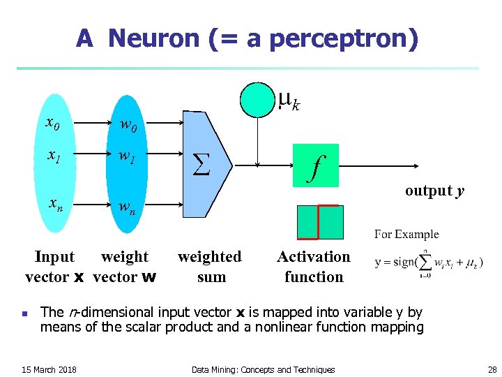A Neuron (= a perceptron) x 0 w 0 x 1 w 1 xn å f wn Input weight vector x vector w n - mk weighted sum output y Activation function The n-dimensional input vector x is mapped into variable y by means of the scalar product and a nonlinear function mapping 15 March 2018 Data Mining: Concepts and Techniques 28

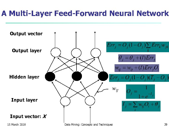A Multi-Layer Feed-Forward Neural Network Output vector Output layer Hidden layer wij Input layer Input vector: X 15 March 2018 Data Mining: Concepts and Techniques 29

How A Multi-Layer Neural Network Works? n n The inputs to the network correspond to the attributes measured for each training tuple Inputs are fed simultaneously into the units making up the input layer n They are then weighted and fed simultaneously to a hidden layer n The number of hidden layers is arbitrary, although usually one n n n The weighted outputs of the last hidden layer are input to units making up the output layer, which emits the network's prediction The network is feed-forward in that none of the weights cycles back to an input unit or to an output unit of a previous layer From a statistical point of view, networks perform nonlinear regression: Given enough hidden units and enough training samples, they can closely approximate any function 15 March 2018 Data Mining: Concepts and Techniques 30

Defining a Network Topology n n n First decide the network topology: # of units in the input layer, # of hidden layers (if > 1), # of units in each hidden layer, and # of units in the output layer Normalizing the input values for each attribute measured in the training tuples to [0. 0— 1. 0] One input unit per domain value, each initialized to 0 Output, if for classification and more than two classes, one output unit per class is used Once a network has been trained and its accuracy is unacceptable, repeat the training process with a different network topology or a different set of initial weights 15 March 2018 Data Mining: Concepts and Techniques 31

Backpropagation n n Iteratively process a set of training tuples & compare the network's prediction with the actual known target value For each training tuple, the weights are modified to minimize the mean squared error between the network's prediction and the actual target value Modifications are made in the “backwards” direction: from the output layer, through each hidden layer down to the first hidden layer, hence “backpropagation” Steps n Initialize weights (to small random #s) and biases in the network n Propagate the inputs forward (by applying activation function) n Backpropagate the error (by updating weights and biases) n Terminating condition (when error is very small, etc. ) 15 March 2018 Data Mining: Concepts and Techniques 32

Backpropagation and Interpretability n n Efficiency of backpropagation: Each epoch (one interation through the training set) takes O(|D| * w), with |D| tuples and w weights, but # of epochs can be exponential to n, the number of inputs, in the worst case Rule extraction from networks: network pruning n n Simplify the network structure by removing weighted links that have the least effect on the trained network Then perform link, unit, or activation value clustering The set of input and activation values are studied to derive rules describing the relationship between the input and hidden unit layers Sensitivity analysis: assess the impact that a given input variable has on a network output. The knowledge gained from this analysis can be represented in rules 15 March 2018 Data Mining: Concepts and Techniques 33

SVM—Support Vector Machines n n n A new classification method for both linear and nonlinear data It uses a nonlinear mapping to transform the original training data into a higher dimension With the new dimension, it searches for the linear optimal separating hyperplane (i. e. , “decision boundary”) With an appropriate nonlinear mapping to a sufficiently high dimension, data from two classes can always be separated by a hyperplane SVM finds this hyperplane using support vectors (“essential” training tuples) and margins (defined by the support vectors) 15 March 2018 Data Mining: Concepts and Techniques 34

SVM—General Philosophy Small Margin Large Margin Support Vectors 15 March 2018 Data Mining: Concepts and Techniques 35

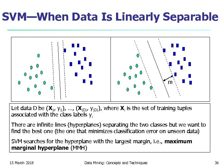SVM—When Data Is Linearly Separable m Let data D be (X 1, y 1), …, (X|D|, y|D|), where Xi is the set of training tuples associated with the class labels yi There are infinite lines (hyperplanes) separating the two classes but we want to find the best one (the one that minimizes classification error on unseen data) SVM searches for the hyperplane with the largest margin, i. e. , maximum marginal hyperplane (MMH) 15 March 2018 Data Mining: Concepts and Techniques 36

SVM—Linearly Separable n A separating hyperplane can be written as W●X+b=0 where W={w 1, w 2, …, wn} is a weight vector and b a scalar (bias) n For 2 -D it can be written as w 0 + w 1 x 1 + w 2 x 2 = 0 n The hyperplane defining the sides of the margin: H 1 : w 0 + w 1 x 1 + w 2 x 2 ≥ 1 for yi = +1, and H 2: w 0 + w 1 x 1 + w 2 x 2 ≤ – 1 for yi = – 1 n n Any training tuples that fall on hyperplanes H 1 or H 2 (i. e. , the sides defining the margin) are support vectors This becomes a constrained (convex) quadratic optimization problem: Quadratic objective function and linear constraints Quadratic Programming (QP) Lagrangian multipliers 15 March 2018 Data Mining: Concepts and Techniques 37

Why Is SVM Effective on High Dimensional Data? n The complexity of trained classifier is characterized by the # of support vectors rather than the dimensionality of the data n The support vectors are the essential or critical training examples — they lie closest to the decision boundary (MMH) n If all other training examples are removed and the training is repeated, the same separating hyperplane would be found n The number of support vectors found can be used to compute an (upper) bound on the expected error rate of the SVM classifier, which is independent of the data dimensionality n Thus, an SVM with a small number of support vectors can have good generalization, even when the dimensionality of the data is high 15 March 2018 Data Mining: Concepts and Techniques 38

SVM vs. Neural Network n SVM n n Relatively new concept n Deterministic algorithm n n n Nice Generalization properties Hard to learn – learned in batch mode using quadratic programming techniques Using kernels can learn very complex functions 15 March 2018 Neural Network n Relatively old n Nondeterministic algorithm n Generalizes well but doesn’t have strong mathematical foundation n Can easily be learned in incremental fashion n To learn complex functions—use multilayer perceptron (not that trivial) Data Mining: Concepts and Techniques 39

Typical Associative Classification Methods n CBA (Classification By Association: Liu, Hsu & Ma, KDD’ 98) n Mine association possible rules in the form of n n n Build classifier: Organize rules according to decreasing precedence based on confidence and then support CMAR (Classification based on Multiple Association Rules: Li, Han, Pei, ICDM’ 01 ) n n Cond-set (a set of attribute-value pairs) class label Classification: Statistical analysis on multiple rules CPAR (Classification based on Predictive Association Rules: Yin & Han, SDM’ 03 ) n n n Generation of predictive rules (FOIL-like analysis) High efficiency, accuracy similar to CMAR RCBT (Mining top-k covering rule groups for gene expression data, Cong et al. SIGMOD’ 05 ) n Explore high-dimensional classification, using top-k rule groups n Achieve high classification accuracy and high run-time efficiency 15 March 2018 Data Mining: Concepts and Techniques 40

A Closer Look at CMAR n n CMAR (Classification based on Multiple Association Rules: Li, Han, Pei, ICDM’ 01 ) Efficiency: Uses an enhanced FP-tree that maintains the distribution of class labels among tuples satisfying each frequent itemset Rule pruning whenever a rule is inserted into the tree n Given two rules, R 1 and R 2, if the antecedent of R 1 is more general than that of R 2 and conf(R 1) ≥ conf(R 2), then R 2 is pruned n Prunes rules for which the rule antecedent and class are not positively correlated, based on a χ2 test of statistical significance Classification based on generated/pruned rules n If only one rule satisfies tuple X, assign the class label of the rule n If a rule set S satisfies X, CMAR n divides S into groups according to class labels 2 n uses a weighted χ measure to find the strongest group of rules, based on the statistical correlation of rules within a group n assigns X the class label of the strongest group 15 March 2018 Data Mining: Concepts and Techniques 41

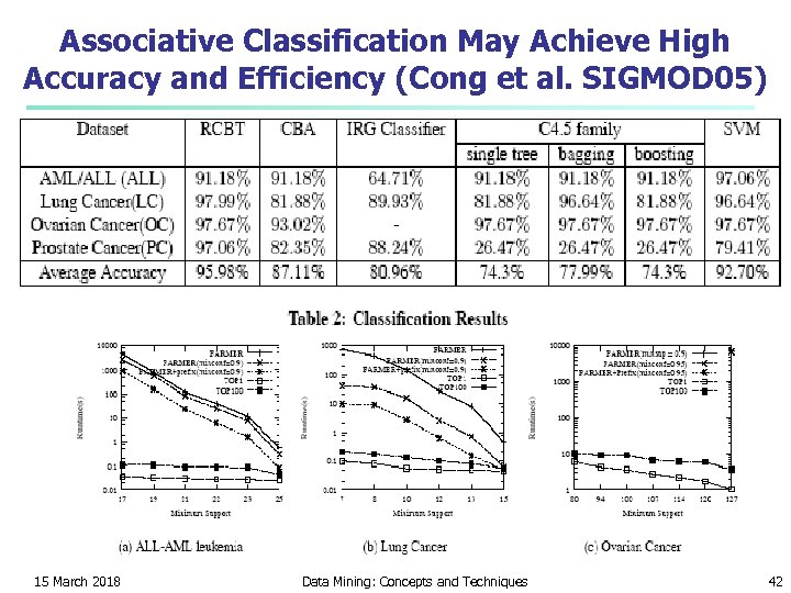Associative Classification May Achieve High Accuracy and Efficiency (Cong et al. SIGMOD 05) 15 March 2018 Data Mining: Concepts and Techniques 42

Lazy vs. Eager Learning n n n Lazy vs. eager learning n Lazy learning (e. g. , instance-based learning): Simply stores training data (or only minor processing) and waits until it is given a test tuple n Eager learning (the above discussed methods): Given a set of training set, constructs a classification model before receiving new (e. g. , test) data to classify Lazy: less time in training but more time in predicting Accuracy n Lazy method effectively uses a richer hypothesis space since it uses many local linear functions to form its implicit global approximation to the target function n Eager: must commit to a single hypothesis that covers the entire instance space 15 March 2018 Data Mining: Concepts and Techniques 43

Lazy Learner: Instance-Based Methods n n Instance-based learning: n Store training examples and delay the processing (“lazy evaluation”) until a new instance must be classified Typical approaches n k-nearest neighbor approach n Instances represented as points in a Euclidean space. n Locally weighted regression n Constructs local approximation n Case-based reasoning n Uses symbolic representations and knowledgebased inference 15 March 2018 Data Mining: Concepts and Techniques 44

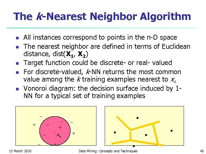The k-Nearest Neighbor Algorithm n n n All instances correspond to points in the n-D space The nearest neighbor are defined in terms of Euclidean distance, dist(X 1, X 2) Target function could be discrete- or real- valued For discrete-valued, k-NN returns the most common value among the k training examples nearest to xq Vonoroi diagram: the decision surface induced by 1 NN for a typical set of training examples _ _ + _ _ 15 March 2018 _. + + xq . _ + . . Data Mining: Concepts and Techniques . . 45

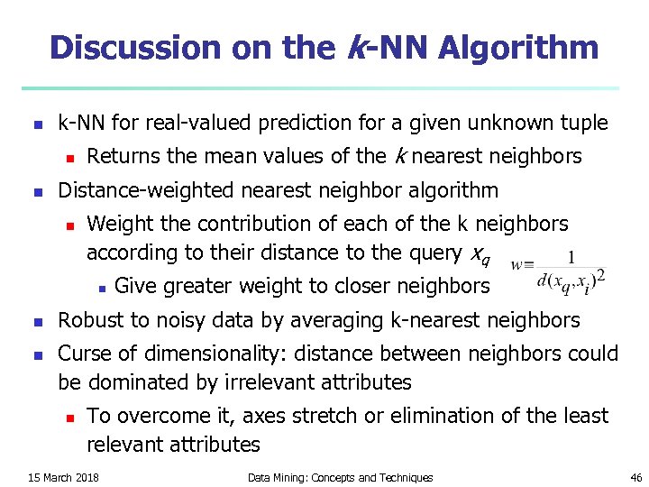Discussion on the k-NN Algorithm n k-NN for real-valued prediction for a given unknown tuple n n Returns the mean values of the k nearest neighbors Distance-weighted nearest neighbor algorithm n Weight the contribution of each of the k neighbors according to their distance to the query xq n n n Give greater weight to closer neighbors Robust to noisy data by averaging k-nearest neighbors Curse of dimensionality: distance between neighbors could be dominated by irrelevant attributes n To overcome it, axes stretch or elimination of the least relevant attributes 15 March 2018 Data Mining: Concepts and Techniques 46

Case-Based Reasoning (CBR) n n CBR: Uses a database of problem solutions to solve new problems Store symbolic description (tuples or cases)—not points in a Euclidean space n Applications: Customer-service (product-related diagnosis), legal ruling n Methodology n n Instances represented by rich symbolic descriptions (e. g. , function graphs) Search for similar cases, multiple retrieved cases may be combined Tight coupling between case retrieval, knowledge-based reasoning, and problem solving Challenges n n Find a good similarity metric Indexing based on syntactic similarity measure, and when failure, backtracking, and adapting to additional cases 15 March 2018 Data Mining: Concepts and Techniques 47

Genetic Algorithms (GA) n Genetic Algorithm: based on an analogy to biological evolution n An initial population is created consisting of randomly generated rules n n n E. g. , if A 1 and ¬A 2 then C 2 can be encoded as 100 n n Each rule is represented by a string of bits If an attribute has k > 2 values, k bits can be used Based on the notion of survival of the fittest, a new population is formed to consist of the fittest rules and their offsprings The fitness of a rule is represented by its classification accuracy on a set of training examples n Offsprings are generated by crossover and mutation n The process continues until a population P evolves when each rule in P satisfies a prespecified threshold n Slow but easily parallelizable 15 March 2018 Data Mining: Concepts and Techniques 48

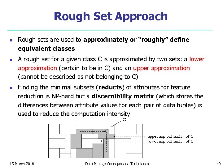Rough Set Approach n n n Rough sets are used to approximately or “roughly” define equivalent classes A rough set for a given class C is approximated by two sets: a lower approximation (certain to be in C) and an upper approximation (cannot be described as not belonging to C) Finding the minimal subsets (reducts) of attributes for feature reduction is NP-hard but a discernibility matrix (which stores the differences between attribute values for each pair of data tuples) is used to reduce the computation intensity 15 March 2018 Data Mining: Concepts and Techniques 49

Evaluating the Accuracy of a Classifier or Predictor (I) n n Holdout method n Given data is randomly partitioned into two independent sets n Training set (e. g. , 2/3) for model construction n Test set (e. g. , 1/3) for accuracy estimation n Random sampling: a variation of holdout n Repeat holdout k times, accuracy = avg. of the accuracies obtained Cross-validation (k-fold, where k = 10 is most popular) n Randomly partition the data into k mutually exclusive subsets, each approximately equal size n At i-th iteration, use Di as test set and others as training set n Leave-one-out: k folds where k = # of tuples, for small sized data n Stratified cross-validation: folds are stratified so that class dist. in each fold is approx. the same as that in the initial data 15 March 2018 Data Mining: Concepts and Techniques 50

Boosting n n Analogy: Consult several doctors, based on a combination of weighted diagnoses—weight assigned based on the previous diagnosis accuracy How boosting works? n Weights are assigned to each training tuple n A series of k classifiers is iteratively learned n n After a classifier Mi is learned, the weights are updated to allow the subsequent classifier, Mi+1, to pay more attention to the training tuples that were misclassified by Mi The final M* combines the votes of each individual classifier, where the weight of each classifier's vote is a function of its accuracy The boosting algorithm can be extended for the prediction of continuous values Comparing with bagging: boosting tends to achieve greater accuracy, but it also risks overfitting the model to misclassified data 15 March 2018 Data Mining: Concepts and Techniques 51

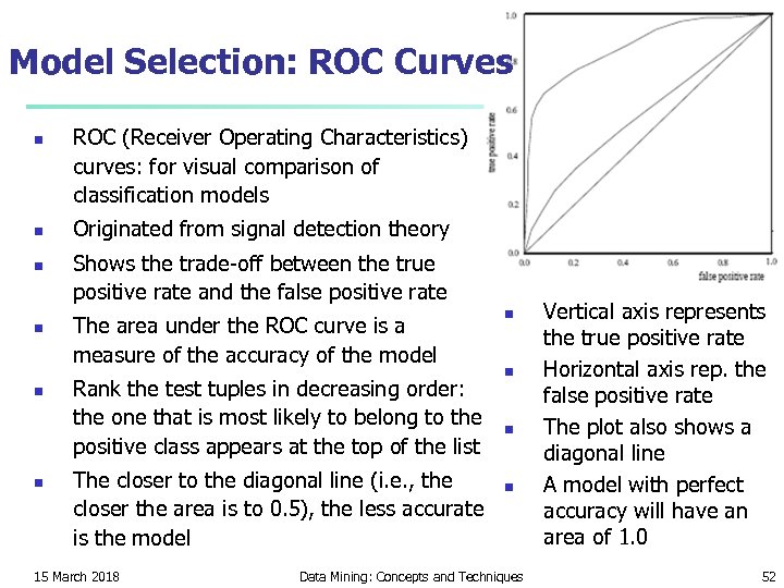Model Selection: ROC Curves n n n ROC (Receiver Operating Characteristics) curves: for visual comparison of classification models Originated from signal detection theory Shows the trade-off between the true positive rate and the false positive rate The area under the ROC curve is a measure of the accuracy of the model Rank the test tuples in decreasing order: the one that is most likely to belong to the positive class appears at the top of the list The closer to the diagonal line (i. e. , the closer the area is to 0. 5), the less accurate is the model 15 March 2018 n n Data Mining: Concepts and Techniques Vertical axis represents the true positive rate Horizontal axis rep. the false positive rate The plot also shows a diagonal line A model with perfect accuracy will have an area of 1. 0 52

Summary (I) n n n Classification and prediction are two forms of data analysis that can be used to extract models describing important data classes or to predict future data trends. Effective and scalable methods have been developed for decision trees induction, Naive Bayesian classification, Bayesian belief network, rule-based classifier, Backpropagation, Support Vector Machine (SVM), associative classification, nearest neighbor classifiers, and case-based reasoning, and other classification methods such as genetic algorithms, rough set and fuzzy set approaches. Linear, nonlinear, and generalized linear models of regression can be used for prediction. Many nonlinear problems can be converted to linear problems by performing transformations on the predictor variables. Regression trees and model trees are also used for prediction. 15 March 2018 Data Mining: Concepts and Techniques 53

Summary (II) n Stratified k-fold cross-validation is a recommended method for accuracy estimation. Bagging and boosting can be used to increase overall accuracy by learning and combining a series of individual models. n Significance tests and ROC curves are useful for model selection n There have been numerous comparisons of the different classification and prediction methods, and the matter remains a research topic n No single method has been found to be superior over all others for all data sets n Issues such as accuracy, training time, robustness, interpretability, and scalability must be considered and can involve trade-offs, further complicating the quest for an overall superior method 15 March 2018 Data Mining: Concepts and Techniques 54