Chapter 5 Transportation Assignment and Network Models

Chapter 5: Transportation, Assignment and Network Models © 2007 Pearson Education

Network Flow Models Consist of a network that can be represented with nodes and arcs 1. Transportation Model 2. Transshipment Model 3. Assignment Model 4. Maximal Flow Model 5. Shortest Path Model 6. Minimal Spanning Tree Model

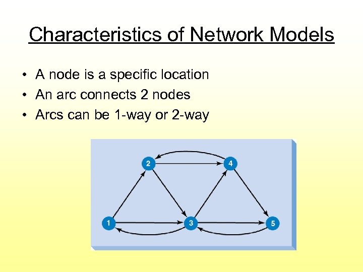Characteristics of Network Models • A node is a specific location • An arc connects 2 nodes • Arcs can be 1 -way or 2 -way

Types of Nodes • Origin nodes • Destination nodes • Transshipment nodes Decision Variables XAB = amount of flow (or shipment) from node A to node B

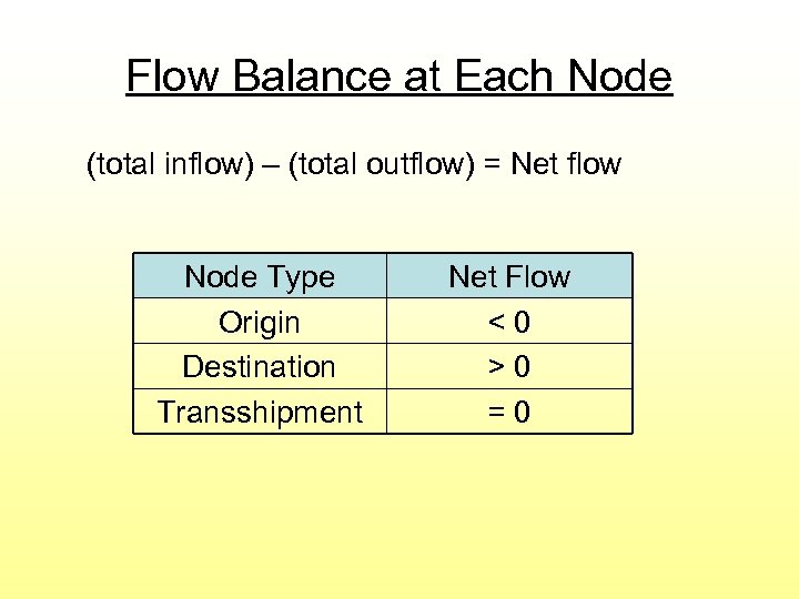Flow Balance at Each Node (total inflow) – (total outflow) = Net flow Node Type Origin Destination Transshipment Net Flow <0 >0 =0

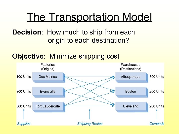The Transportation Model Decision: How much to ship from each origin to each destination? Objective: Minimize shipping cost

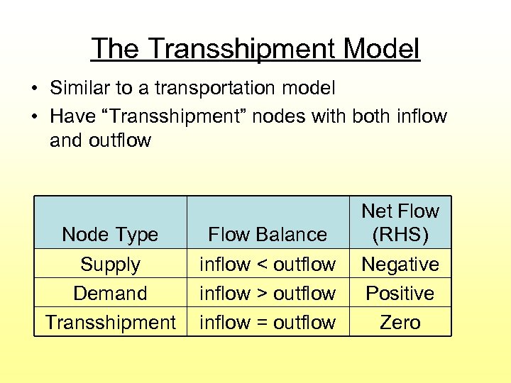The Transshipment Model • Similar to a transportation model • Have “Transshipment” nodes with both inflow and outflow Node Type Supply Demand Transshipment Flow Balance inflow < outflow inflow > outflow inflow = outflow Net Flow (RHS) Negative Positive Zero

Assignment Model • For making one-to-one assignments • Such as: – People to tasks – Classes to classrooms – Etc.

The Maximal-Flow Model Where networks have arcs with limited capacity, such as roads or pipelines Decision: How much flow on each arc? Objective: Maximize flow through the network from an origin to a destination

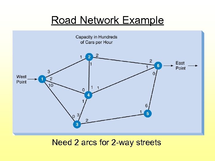Road Network Example Need 2 arcs for 2 -way streets

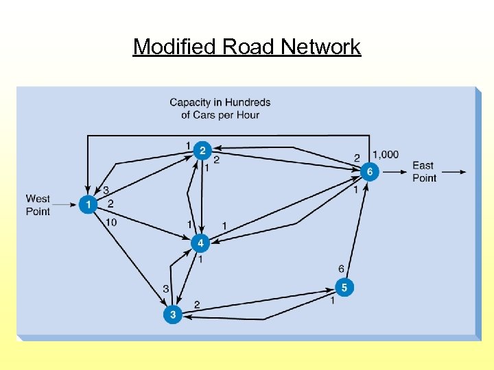Modified Road Network

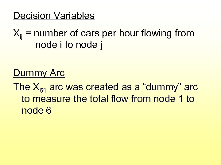Decision Variables Xij = number of cars per hour flowing from node i to node j Dummy Arc The X 61 arc was created as a “dummy” arc to measure the total flow from node 1 to node 6

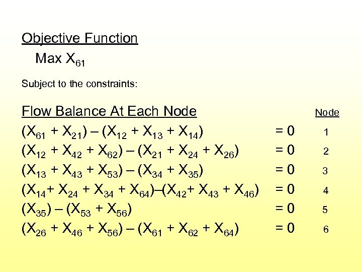Objective Function Max X 61 Subject to the constraints: Flow Balance At Each Node (X 61 + X 21) – (X 12 + X 13 + X 14) (X 12 + X 42 + X 62) – (X 21 + X 24 + X 26) (X 13 + X 43 + X 53) – (X 34 + X 35) (X 14+ X 24 + X 34 + X 64)–(X 42+ X 43 + X 46) (X 35) – (X 53 + X 56) (X 26 + X 46 + X 56) – (X 61 + X 62 + X 64) Node =0 =0 =0 1 2 3 4 5 6

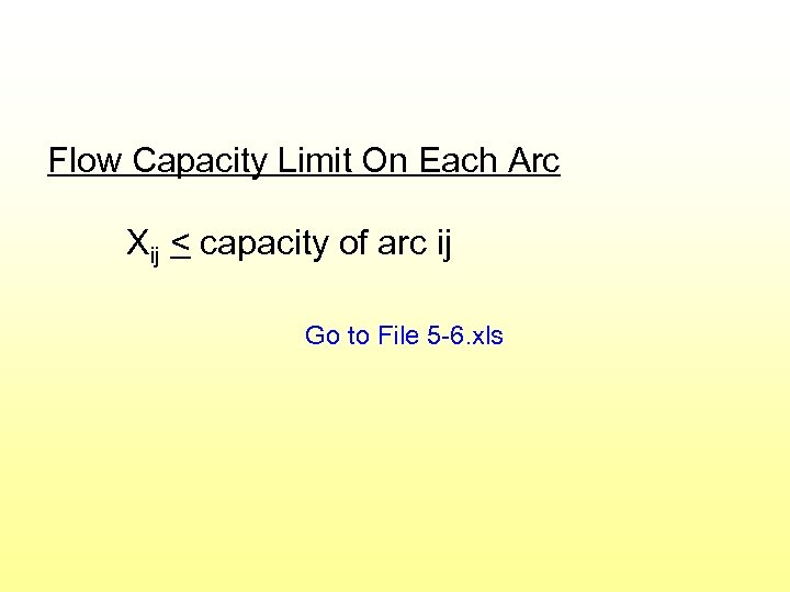Flow Capacity Limit On Each Arc Xij < capacity of arc ij Go to File 5 -6. xls

The Shortest Path Model For determining the shortest distance to travel through a network to go from an origin to a destination Decision: Which arcs to travel on? Objective: Minimize the distance (or time) from the origin to the destination

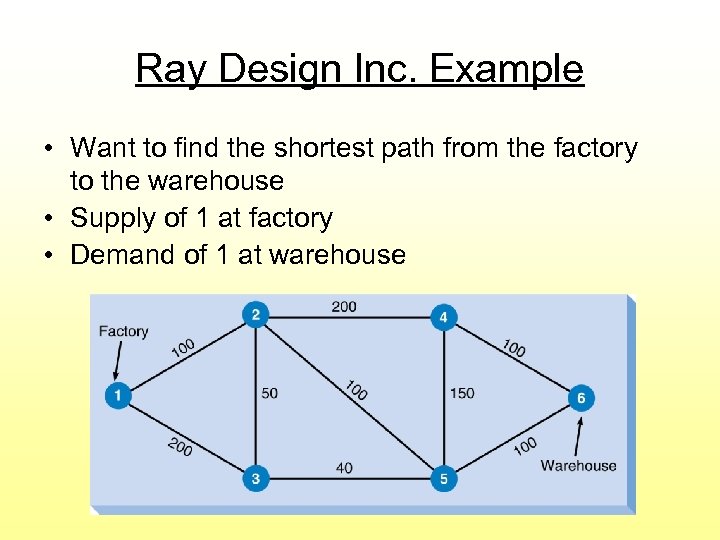Ray Design Inc. Example • Want to find the shortest path from the factory to the warehouse • Supply of 1 at factory • Demand of 1 at warehouse

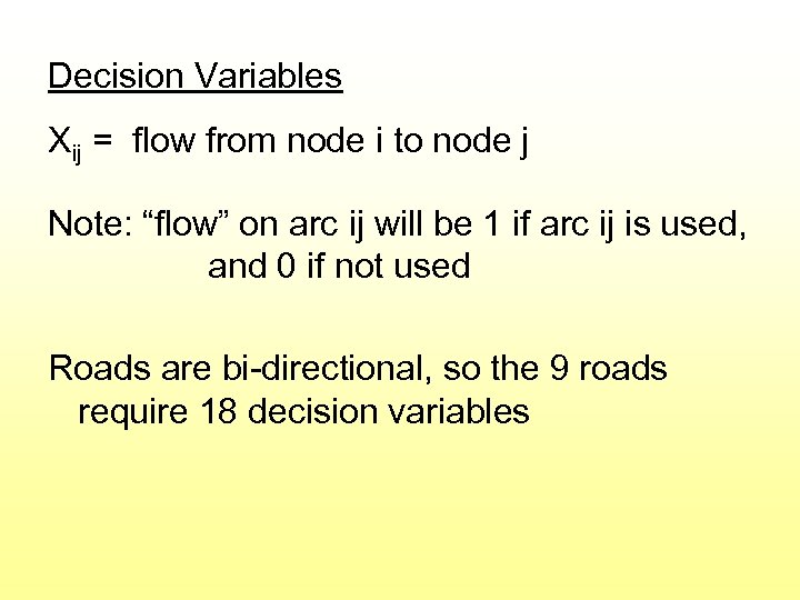Decision Variables Xij = flow from node i to node j Note: “flow” on arc ij will be 1 if arc ij is used, and 0 if not used Roads are bi-directional, so the 9 roads require 18 decision variables

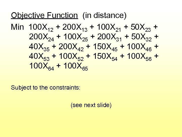Objective Function (in distance) Min 100 X 12 + 200 X 13 + 100 X 21 + 50 X 23 + 200 X 24 + 100 X 25 + 200 X 31 + 50 X 32 + 40 X 35 + 200 X 42 + 150 X 45 + 100 X 46 + 40 X 53 + 100 X 52 + 150 X 54 + 100 X 56 + 100 X 64 + 100 X 65 Subject to the constraints: (see next slide)

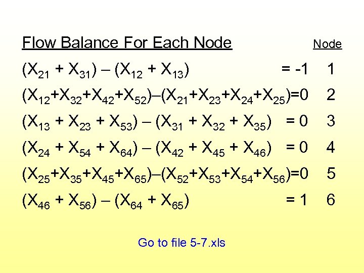Flow Balance For Each Node (X 21 + X 31) – (X 12 + X 13) Node = -1 1 (X 12+X 32+X 42+X 52)–(X 21+X 23+X 24+X 25)=0 2 (X 13 + X 23 + X 53) – (X 31 + X 32 + X 35) = 0 3 (X 24 + X 54 + X 64) – (X 42 + X 45 + X 46) = 0 4 (X 25+X 35+X 45+X 65)–(X 52+X 53+X 54+X 56)=0 5 (X 46 + X 56) – (X 64 + X 65) 6 Go to file 5 -7. xls =1

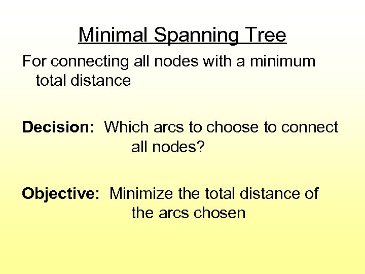Minimal Spanning Tree For connecting all nodes with a minimum total distance Decision: Which arcs to choose to connect all nodes? Objective: Minimize the total distance of the arcs chosen

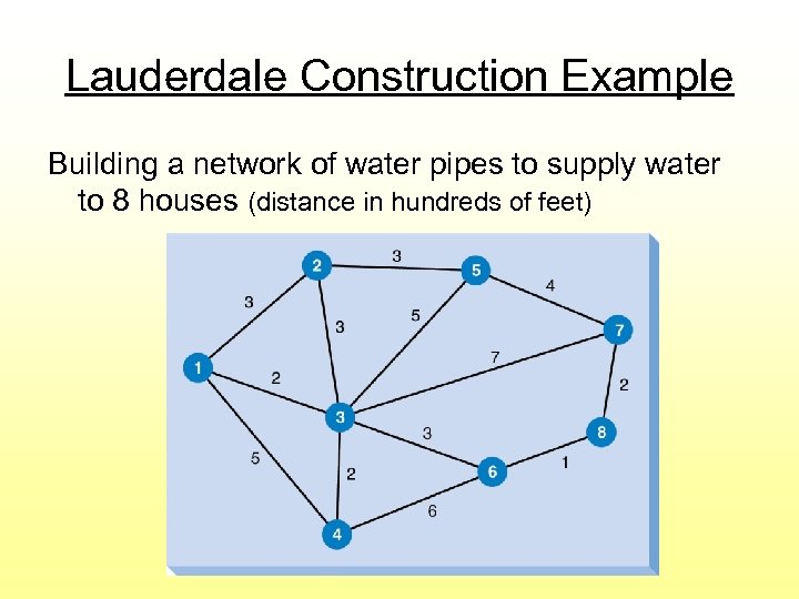Lauderdale Construction Example Building a network of water pipes to supply water to 8 houses (distance in hundreds of feet)

Characteristics of Minimal Spanning Tree Problems • Nodes are not pre-specified as origins or destinations • So we do not formulate as LP model • Instead there is a solution procedure

Steps for Solving Minimal Spanning Tree 1. Select any node 2. Connect this node to its nearest node 3. Find the nearest unconnected node and connect it to the tree (if there is a tie, select one arbitrarily) 4. Repeat step 3 until all nodes are connected

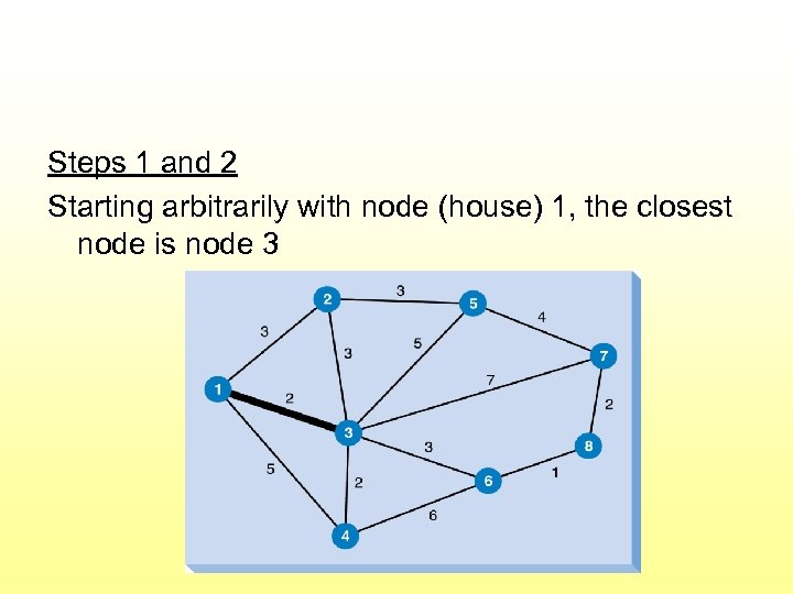Steps 1 and 2 Starting arbitrarily with node (house) 1, the closest node is node 3

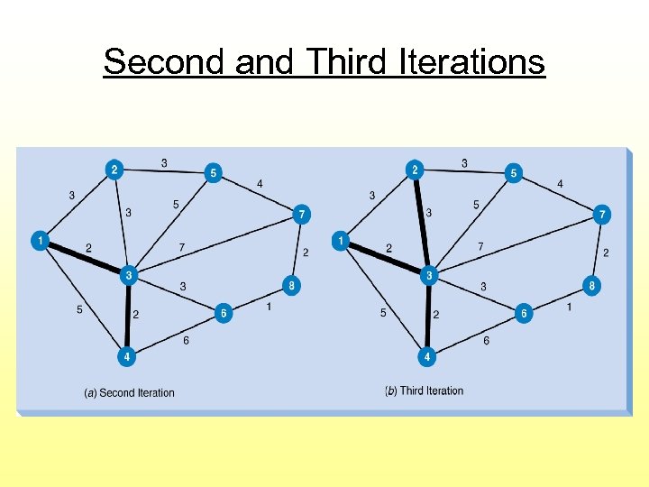Second and Third Iterations

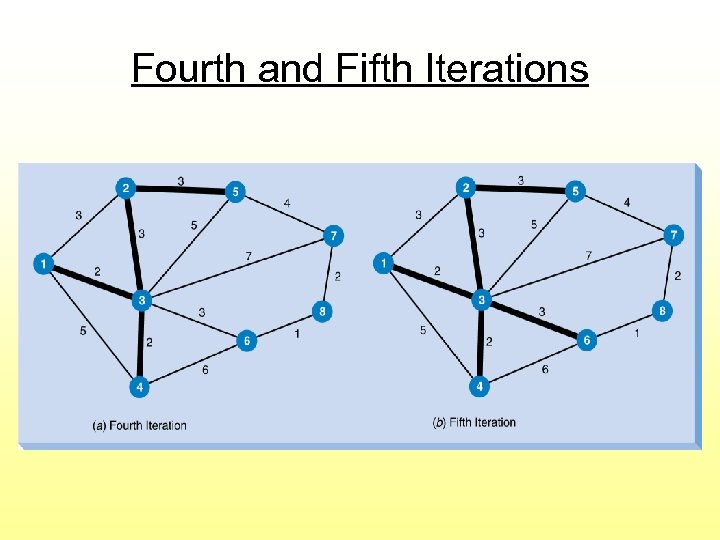Fourth and Fifth Iterations

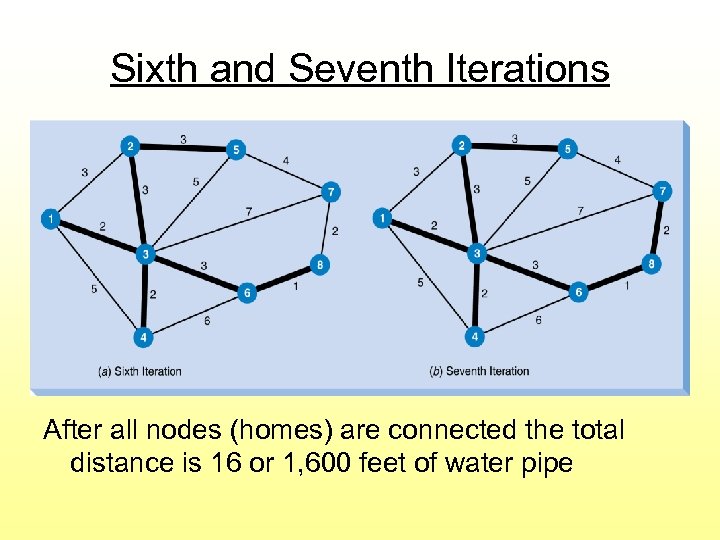Sixth and Seventh Iterations After all nodes (homes) are connected the total distance is 16 or 1, 600 feet of water pipe