Chapter 5 The Value of Information Mc Graw-Hill Irwin

Chapter 5 The Value of Information Mc. Graw-Hill/Irwin Copyright © 2008 by The Mc. Graw-Hill Companies, Inc. All rights reserved.

5. 1 Introduction Value of using any type of information technology l Potential availability of more and more information throughout the supply chain l Implications this availability on effective design and management of the integrated supply chain l 1 -2

Information Types Inventory levels l Orders l Production l Delivery status l 1 -3

More Information l l l Helps reduce variability in the supply chain. Helps suppliers make better forecasts, accounting for promotions and market changes. Enables the coordination of manufacturing and distribution systems and strategies. Enables retailers to better serve their customers by offering tools for locating desired items. Enables retailers to react and adapt to supply problems more rapidly. Enables lead time reductions. 1 -4

5. 2 Bullwhip Effect While customer demand for specific products does not vary much l Inventory and back-order levels fluctuate considerably across their supply chain l P&G’s disposable diapers case l Sales quite flat l Distributor orders fluctuate more than retail sales l Supplier orders fluctuate even more l 1 -5

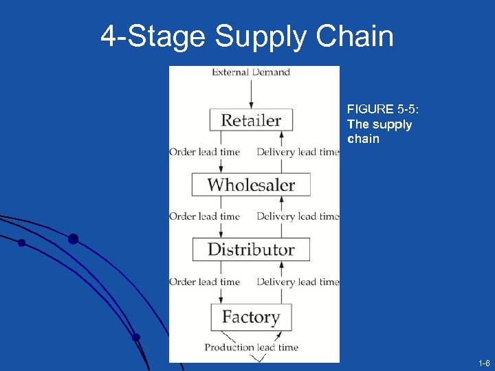4 -Stage Supply Chain FIGURE 5 -5: The supply chain 1 -6

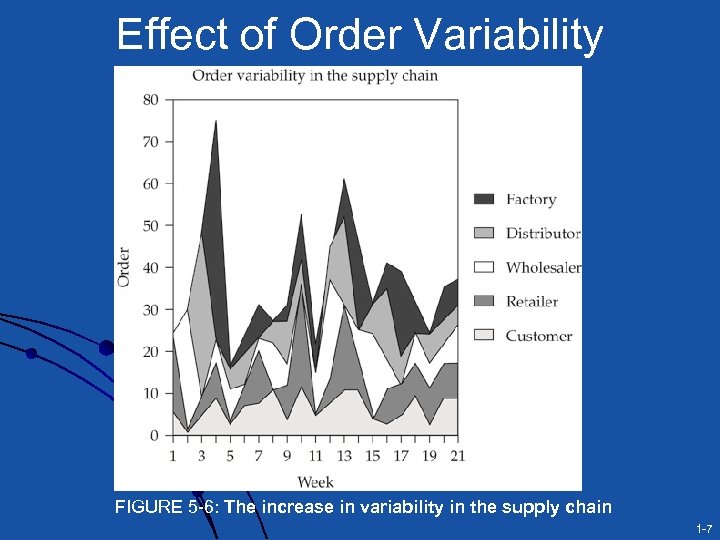Effect of Order Variability FIGURE 5 -6: The increase in variability in the supply chain 1 -7

Factors that Contribute to the Variability - Demand Forecasting l l l l Periodic review policy Characterized by a single parameter, the base-stock level. Base-stock level = Average demand during lead time and review period + a multiple of the standard deviation of demand during lead time and review period (safety stock) Estimation of average demand variability done using standard forecast smoothing techniques. Estimates get modified as more data becomes available Safety stock and base-stock level depends on these estimates Order quantities are changed accordingly increasing variability 1 -8

Factors that Contribute to the Variability – Lead Time l l l Increase in variability magnified with increasing lead time. Safety stock and base-stock levels have a lead time component in their estimations. With longer lead times: l l a small change in the estimate of demand variability implies a significant change in safety stock and base-stock level, which implies significant changes in order quantities leads to an increase in variability 1 -9

Factors that Contribute to the Variability – Batch Ordering l l Retailer uses batch ordering, as with a (Q, R) or a min-max policy Wholesaler observes a large order, followed by several periods of no orders, followed by another large order, and so on. Wholesaler sees a distorted and highly variable pattern of orders. Such pattern is also a result of: l l Transportation discounts with large orders Periodic sales quotas/incentives 1 -10

Factors that Contribute to the Variability – Price Fluctuations l Retailers often attempt to stock up when prices are lower. Accentuated by promotions and discounts at certain times or for certain quantities. l Such Forward Buying results in: l l Large order during the discounts l Relatively small orders at other time periods 1 -11

Factors that Contribute to the Variability – Inflated Orders Inflated orders during shortage periods l Common when retailers and distributors suspect that a product will be in short supply and therefore anticipate receiving supply proportional to the amount ordered. l After period of shortage, retailer goes back to its standard orders l l leads to all kinds of distortions and variations in demand estimates 1 -12

Quantifying the Bullwhip l Consider a two-stage supply chain: l l l Retailer faces a fixed lead time l l l Retailer who observes customer demand Retailer places an order to a manufacturer. order placed at the end of period t Order received at the start of period t+L. Retailer follows a simple periodic review policy l l l retailer reviews inventory every period places an order to bring its inventory level up to a target level. the review period is one 1 -13

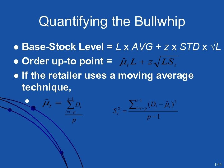Quantifying the Bullwhip Base-Stock Level = L x AVG + z x STD x √L l Order up-to point = l If the retailer uses a moving average technique, l l 1 -14

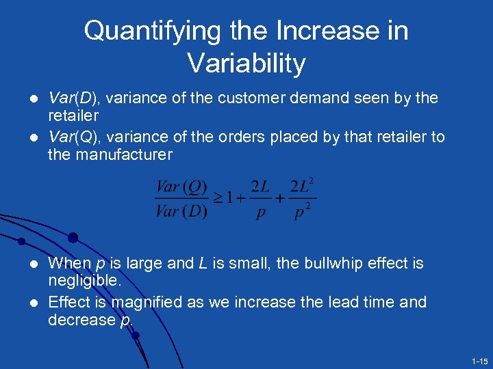Quantifying the Increase in Variability l l Var(D), variance of the customer demand seen by the retailer Var(Q), variance of the orders placed by that retailer to the manufacturer When p is large and L is small, the bullwhip effect is negligible. Effect is magnified as we increase the lead time and decrease p. 1 -15

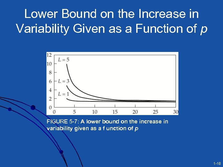Lower Bound on the Increase in Variability Given as a Function of p FIGURE 5 -7: A lower bound on the increase in variability given as a f unction of p 1 -16

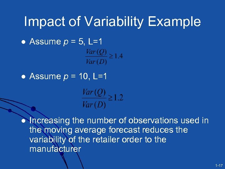Impact of Variability Example l Assume p = 5, L=1 l Assume p = 10, L=1 l Increasing the number of observations used in the moving average forecast reduces the variability of the retailer order to the manufacturer 1 -17

Impact of Centralized Information on Bullwhip Effect l Centralize demand information within a supply chain Provide each stage of supply chain with complete information on the actual customer demand l Creates more accurate forecasts rather than orders received from the previous stage l 1 -18

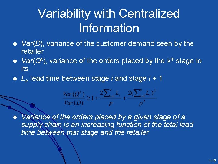Variability with Centralized Information l l Var(D), variance of the customer demand seen by the retailer Var(Qk), variance of the orders placed by the kth stage to its Li, lead time between stage i and stage i + 1 Variance of the orders placed by a given stage of a supply chain is an increasing function of the total lead time between that stage and the retailer 1 -19

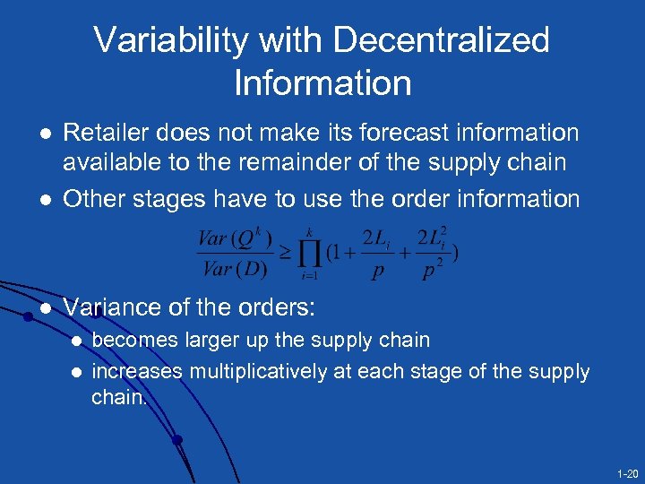Variability with Decentralized Information l Retailer does not make its forecast information available to the remainder of the supply chain Other stages have to use the order information l Variance of the orders: l l l becomes larger up the supply chain increases multiplicatively at each stage of the supply chain. 1 -20

Managerial Insights Variance increases up the supply chain in both centralized and decentralized cases l Variance increases: l Additively with centralized case l Multiplicatively with decentralized case l l Centralizing demand information can significantly reduce the bullwhip effect l Although not eliminate it completely!! 1 -21

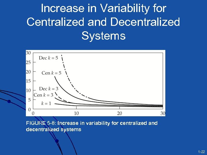Increase in Variability for Centralized and Decentralized Systems FIGURE 5 -8: Increase in variability for centralized and decentralized systems 1 -22

Methods for Coping with the Bullwhip l Reducing uncertainty. Centralizing information l Reducing variability inherent in the customer demand process. l “Everyday low pricing” (EDLP) strategy. l 1 -23

Methods for Coping with the Bullwhip l Lead-time reduction l l Lead times magnify the increase in variability due to demand forecasting. Two components of lead times: l l l order lead times [can be reduced through the use of crossdocking] Information lead times [can be reduced through the use of electronic data interchange (EDI). ] Strategic partnerships l l Changing the way information is shared and inventory is managed Vendor managed inventory (VMI) l l Manufacturer manages the inventory of its product at the retailer outlet VMI the manufacturer does not rely on the orders placed by a retailer, thus avoiding the bullwhip effect entirely. 1 -24

5. 3 Information Sharing And Incentives l l l Centralizing information will reduce variability Upstream stages would benefit more Unfortunately, information sharing is a problem in many industries Inflated forecasts are a reality Forecast information is inaccurate and distorted l l Forecasts inflated such that suppliers build capacity Suppliers may ignore the forecasts totally 1 -25

Contractual Incentives to Get True Forecasts from Buyers l Capacity Reservation Contract l l Buyer pays to reserve a certain level of capacity at the supplier A menu of prices for different capacity reservations provided by supplier Buyer signals true forecast by reserving a specific capacity level Advance Purchase Contract l l l Supplier charges special price before building capacity When demand is realized, price charged is different Buyer’s commitment to paying the special price reveals the buyer’s true forecast 1 -26

5. 4 Effective Forecasts l Retailer forecasts l l Distributor and manufacturer forecasts l l l Typically based on an analysis of previous sales at the retailer. Future customer demand influenced by pricing, promotions, and release of new products. Including such information will make forecasts more accurate. Influenced by factors under retailer control. Promotions or pricing. Retailer may introduce new products into the stores Closer to actual sales – may have more information Cooperative forecasting systems l l Sophisticated information systems iterative forecasting process all participants in the supply chain collaborate to arrive at an agreed-upon forecast All parties share and use the same forecasting tool 1 -27

5. 5 Information for the Coordination of Systems l Many interconnected systems l l l manufacturing, storage, transportation, and retail systems the outputs from one system within the supply chain are the inputs to the next system trying to find the best set of trade-offs for any one stage isn’t sufficient. need to consider the entire system and coordinate decisions Systems are not coordinated l l each facility in the supply chain does what is best for that facility the result is local optimization. 1 -28

Global Optimization l Issues: Who will optimize? l How will the savings obtained through the coordinated strategy be split between the different supply chain facilities? l l Methods to address issues: Supply contracts l Strategic partnerships l 1 -29

5. 6 Locating Desired Products l l Meet customer demand from available retailer inventory What if the item is not in stock at the retailer? l l l Being able to locate and deliver goods is sometimes as effective as having them in stock If the item is available at the competitor, then this is a problem Other Methods l l Inventory pooling (Chapter 7) Distributor Integration (Chapter 8) 1 -30

5. 7 Lead-Time Reduction l Numerous benefits: l l l l The ability to quickly fill customer orders that can’t be filled from stock. Reduction in the bullwhip effect. More accurate forecasts due to a decreased forecast horizon. Reduction in finished goods inventory levels Many firms actively look for suppliers with shorter lead times Many potential customers consider lead time a very important criterion for vendor selection. Much of the manufacturing revolution of the past 20 years led to reduced lead times Other methods: l l l Distribution network designs (Chapter 6) Effective information systems (e. g. , EDI) Strategic partnering (Chapter 8) (Sharing point-of-sale (POS) data with supplier) 1 -31

5. 8 Information and Supply Chain Trade-Offs Conflicting objectives in the supply chains l Designing the supply chain with conflicting goals l 1 -32

Wish-Lists of the Different Stages l Raw material suppliers l l Manufacturing l l l Minimizing transportation costs through: quantity discounts, minimizing inventory levels, quickly replenishing stock. Retailers l l High productivity through production efficiencies and low production costs Known future demand pattern with little variability. Materials, warehousing, and outbound logistics l l Stable volume requirements and little variation in mix Flexible delivery times Large volume demands Short order lead times and efficient, accurate order delivery Customers l In-stock items, enormous variety, and low prices. 1 -33

Trade-Offs: Inventory-Lot Size l Manufacturers would like to have large lot sizes. l l Modern practices [Setup time reduction, Kanban and CONWIP] l l Per unit setup costs are reduced Manufacturing expertise for a particular product increases Processes are easier to control. Reduce inventories and improve system responsiveness. Advanced manufacturing systems make it possible for manufacturers to meet shorter lead times and respond more rapidly to customer needs. Manufacturer should have as much time as possible to react to the needs of downstream supply chain members. Distributors/retailers can have factory status and manufacturer inventory data: l l l they can quote lead times to customers more accurately. develops an understanding of, and confidence in, the manufacturers’ ability. allows reduction in inventory in anticipation of manufacturing problems 1 -34

Trade-offs Inventory-Transportation Costs l Company operates its own fleet of trucks. l l l Outside firm is used for shipping l l l quantity discounts TL shipping cheaper than LTL shipping In many cases l l l Fixed cost of operation + variable cost Carrying full truckloads minimizes transportation costs. demand is much less than TL Items sit for a long time before consumption leading to higher inventory costs. Trade-off can’t be eliminated completely. l l Use advanced information technology to reduce this effect. Distribution control systems allow combining shipments of different products from warehouses to stores Cross-docking, Decision-support systems allow appropriate balance between transportation and inventory costs 1 -35

Trade-offs Lead Time-Transportation Costs l Transportation costs lowest when large quantities of items are transported between stages of the supply chain. l l l Hold items to accumulate enough to combine shipments Lead times can be reduced if items are transported immediately after they are manufactured or arrive from suppliers. Cannot be completely eliminated l l l Information can be used to reduce its effect. Control transportation costs reducing the need to hold items until a sufficient number accumulate. Improved forecasting techniques and information systems reduce the other components of lead time l may not be essential to reduce the transportation component. 1 -36

Trade-Offs Product Variety-Inventory l Higher product variety makes supply chain decisions more complex Better for meeting customer demand l Typically leads to higher inventories l l Strategies: l Delayed Differentiation (Chapter 6) l Ship generic products as far as possible down the supply chain l Design for logistics (Chapter 11) 1 -37

Trade-Offs Cost-Customer Service l l l Reducing inventories, manufacturing costs, and transportation costs typically comes at the expense of customer service Customer service could mean the ability of a retailer to meet a customer’s demand quickly Strategies: l l l transshipping direct shipping from warehouses to customers Charging price premiums for customized products 1 -38

5. 9 Decreasing Marginal Value of Information l l l Obtaining and sharing information is not free. Many firms are struggling with exactly how to use the data they collect through loyalty programs, RFID readers, and so on. Cost of exchanging information versus the benefit of doing so. l l May not be necessary to exchange all of the available information, or to exchange information continuously. Decreasing marginal value of additional information In multi-stage decentralized manufacturing supply chains many of the performance benefits of detailed information sharing can be achieved if only a small amount of information is exchanged between supply chain participants. Exchanging more detailed information or more frequent information is costly. l l l Understand the costs and benefits of particular pieces of information How often this information is collected How much of this information needs to be stored How much of this information needs to be shared In what form it needs to shared 1 -39

Summary l l l The bullwhip effect suggests that variability in demand increases as one moves up in the supply chain. Increase in variability causes significant operational inefficiencies Specific techniques to “counteract” bullwhip effect l l Information sharing, i. e. , centralized demand information. Incentives to share credible forecasts Alignments of expectations associated with the use of information. Interaction of various supply chain stages. l l l A series of trade-offs both within and between the different stages. Information is the key enabler of integrating the different supply chain stages Information can be used to reduce the necessity of many of these trade-offs 1 -40

CASE: Reebok NFL Replica Jerseys: A Case for Postponement Stephen C. Graves, John C. W. Parsons MIT, Cambridge MA, USA Mc. Kinsey & Co. , Toronto, Ontario, Canada 1 -41

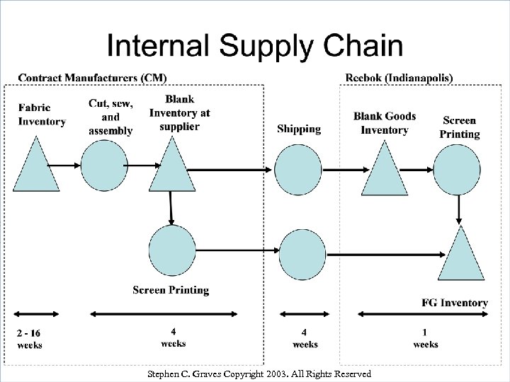
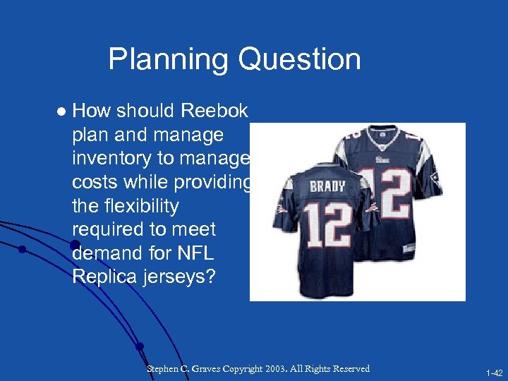Planning Question l How should Reebok plan and manage inventory to manage costs while providing the flexibility required to meet demand for NFL Replica jerseys? Stephen C. Graves Copyright 2003. All Rights Reserved 1 -42

Outline of Case Discussion • Discuss business context, nature of demand, the sales cycle, key success factors, failure modes • Discuss supply chain, planning cycle, planning challenges • Frame as single-season planning problem; relate to newsvendor model • Develop approach and key insights with NE Patriots example • Report on findings for NFL • Wrap up and summary of learnings Stephen C. Graves Copyright 2003. All Rights Reserved 1 -43

Licensed Apparel Business Situation Impact l Reebok received an NFL exclusive license in 2000 l No direct competition for product – 100% market share l Highly seasonal & very uncertain demand for player jerseys l Demand is concentrated over five month period l Teams are more predictable, but correlated with success l l Hot-market players and teams emerge during season If product is not quickly available to meet demand the opportunity is lost l Lost sales cost more than inventory overstocks, but come with a high risk of obsolescence l High margins, fashion item l Demand driven by availability l Unsold jerseys can become instantly obsolete – trades; design changes Stephen C. Graves Copyright 2003. All Rights Reserved 1 -44

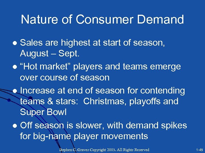Nature of Consumer Demand Sales are highest at start of season, August – Sept. l “Hot market” players and teams emerge over course of season l Increase at end of season for contending teams & stars: Christmas, playoffs and Super Bowl l Off season is slower, with demand spikes for big-name player movements l Stephen C. Graves Copyright 2003. All Rights Reserved 1 -45

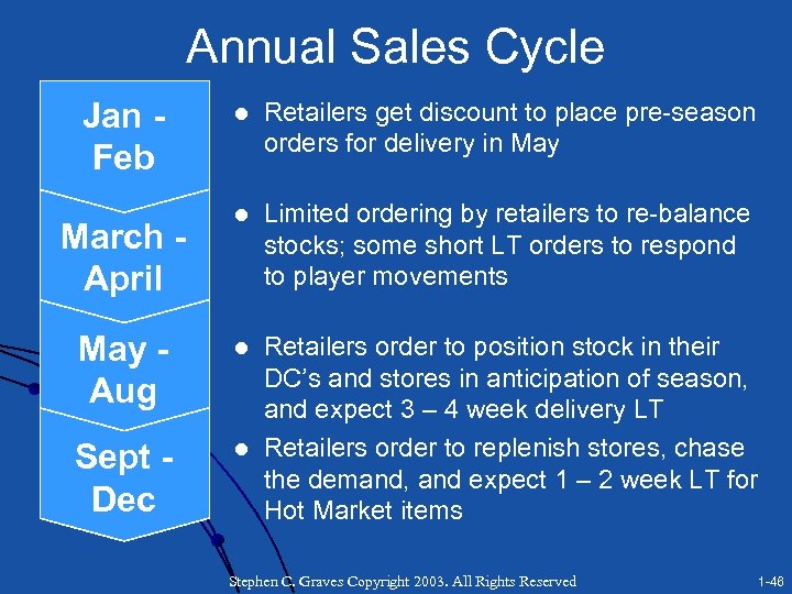Annual Sales Cycle Jan Feb l Retailers get discount to place pre-season orders for delivery in May l Limited ordering by retailers to re-balance stocks; some short LT orders to respond to player movements May Aug l Sept Dec l Retailers order to position stock in their DC’s and stores in anticipation of season, and expect 3 – 4 week delivery LT Retailers order to replenish stores, chase the demand, and expect 1 – 2 week LT for Hot Market items March April Stephen C. Graves Copyright 2003. All Rights Reserved 1 -46

Outline of Case Discussion l l l Discuss business context, nature of demand, the sales cycle, key success factors, failure modes Discuss supply chain, planning cycle, planning challenges Frame as single-season planning problem; relate to newsvendor model Develop approach and key insights with NE Patriots example Report on findings for NFL Wrap up and summary of learnings Stephen C. Graves Copyright 2003. All Rights Reserved 1 -47

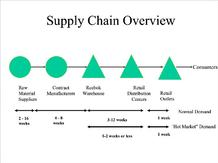Stephen C. Graves Copyright 2003. All Rights Reserved 1 -48

Stephen C. Graves Copyright 2003. All Rights Reserved 1 -49

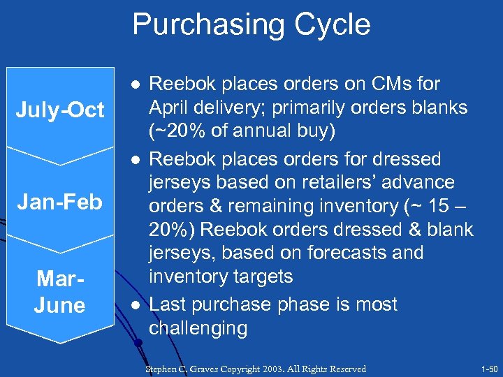Purchasing Cycle l July-Oct l Jan-Feb Mar. June l Reebok places orders on CMs for April delivery; primarily orders blanks (~20% of annual buy) Reebok places orders for dressed jerseys based on retailers’ advance orders & remaining inventory (~ 15 – 20%) Reebok orders dressed & blank jerseys, based on forecasts and inventory targets Last purchase phase is most challenging Stephen C. Graves Copyright 2003. All Rights Reserved 1 -50

Outline of Case Discussion l l l Discuss business context, nature of demand, the sales cycle, key success factors, failure modes Discuss supply chain, planning cycle, planning challenges Frame as single-season planning problem; relate to newsvendor model Develop approach and key insights with NE Patriots example Report on findings for NFL Wrap up and summary of learnings Stephen C. Graves Copyright 2003. All Rights Reserved 1 -51

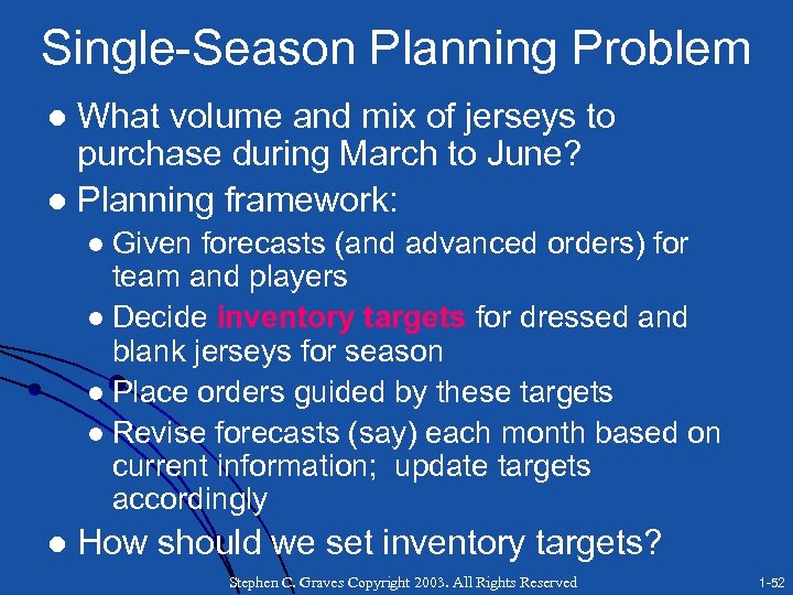Single-Season Planning Problem What volume and mix of jerseys to purchase during March to June? l Planning framework: l Given forecasts (and advanced orders) for team and players l Decide inventory targets for dressed and blank jerseys for season l Place orders guided by these targets l Revise forecasts (say) each month based on current information; update targets accordingly l l How should we set inventory targets? Stephen C. Graves Copyright 2003. All Rights Reserved 1 -52

Outline of Case Discussion l l l Discuss business context, nature of demand, the sales cycle, key success factors, failure modes Discuss supply chain, planning cycle, planning challenges Frame as single-season planning problem; relate to newsvendor model Develop approach and key insights with NE Patriots example Report on findings for NFL Wrap up and summary of learnings Stephen C. Graves Copyright 2003. All Rights Reserved 1 -53

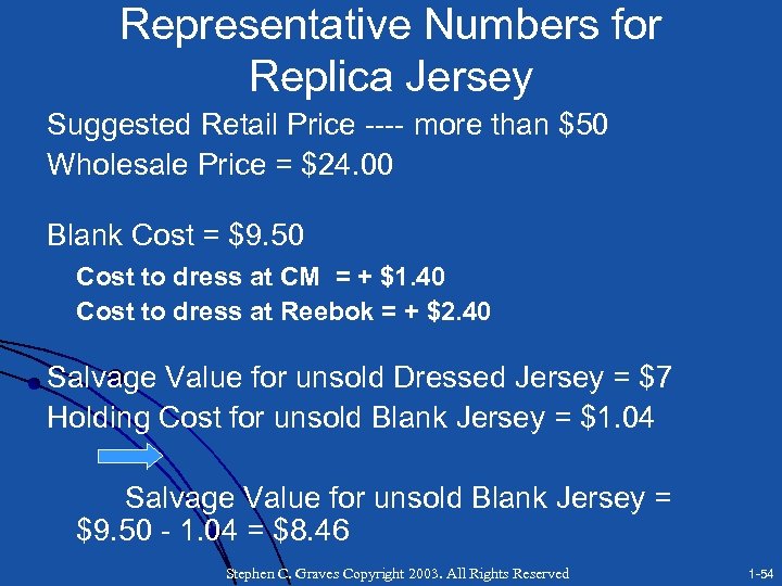Representative Numbers for Replica Jersey Suggested Retail Price ---- more than $50 Wholesale Price = $24. 00 Blank Cost = $9. 50 Cost to dress at CM = + $1. 40 Cost to dress at Reebok = + $2. 40 Salvage Value for unsold Dressed Jersey = $7 Holding Cost for unsold Blank Jersey = $1. 04 Salvage Value for unsold Blank Jersey = $9. 50 - 1. 04 = $8. 46 Stephen C. Graves Copyright 2003. All Rights Reserved 1 -54

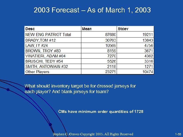2003 Forecast – As of March 1, 2003 What should inventory target be for dressed jerseys for each player? And blank jerseys for team? CMs have minimum order quantities of 1728 Stephen C. Graves Copyright 2003. All Rights Reserved 1 -55

What’s the Objective? l Expected revenue: l $24*E[Dressed_Sold] + 24*E[Blanks_Sold] + $7*E[Dressed_Unsold] + $8. 46* E[Blanks_Unsold] l Expected Cost: l $9. 50*Blanks + $10. 90*Dressed + $2. 40*E[Blanks_Sold] Stephen C. Graves Copyright 2003. All Rights Reserved 1 -56

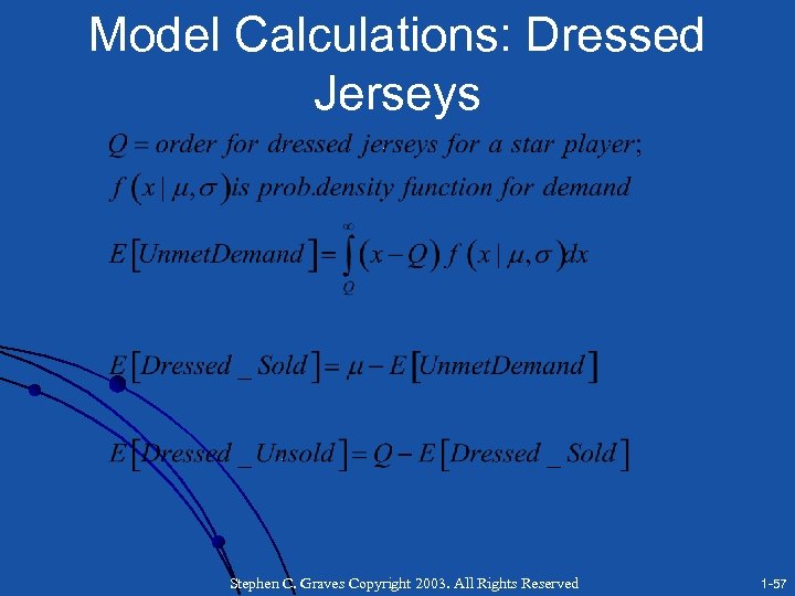Model Calculations: Dressed Jerseys Stephen C. Graves Copyright 2003. All Rights Reserved 1 -57

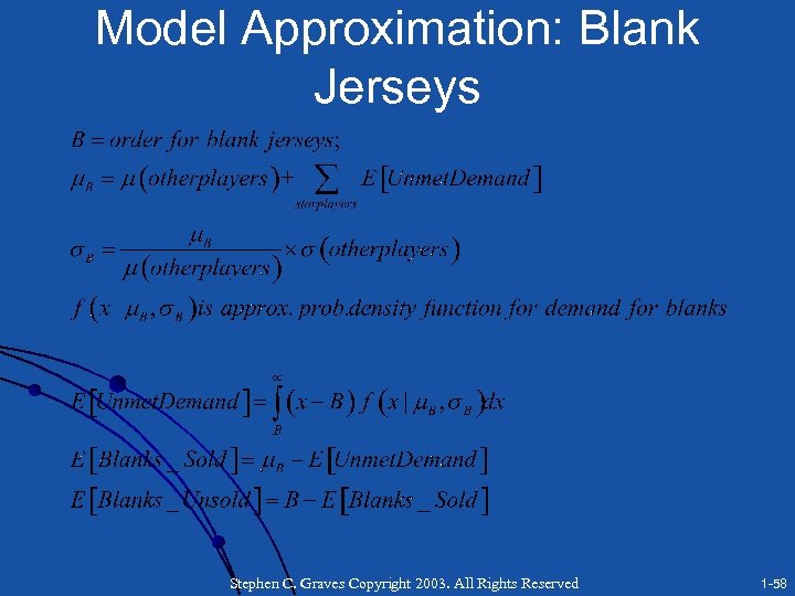Model Approximation: Blank Jerseys Stephen C. Graves Copyright 2003. All Rights Reserved 1 -58

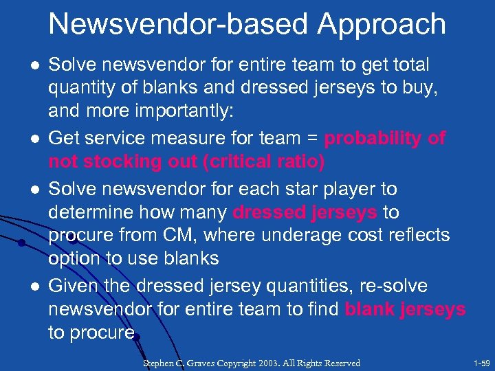Newsvendor-based Approach l l Solve newsvendor for entire team to get total quantity of blanks and dressed jerseys to buy, and more importantly: Get service measure for team = probability of not stocking out (critical ratio) Solve newsvendor for each star player to determine how many dressed jerseys to procure from CM, where underage cost reflects option to use blanks Given the dressed jersey quantities, re-solve newsvendor for entire team to find blank jerseys to procure Stephen C. Graves Copyright 2003. All Rights Reserved 1 -59

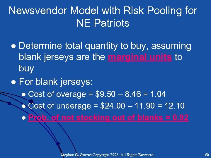Newsvendor Model with Risk Pooling for NE Patriots Determine total quantity to buy, assuming blank jerseys are the marginal units to buy l For blank jerseys: l Cost of overage = $9. 50 – 8. 46 = 1. 04 l Cost of underage = $24. 00 – 11. 90 = 12. 10 l Prob. of not stocking out of blanks = 0. 92 l Stephen C. Graves Copyright 2003. All Rights Reserved 1 -60

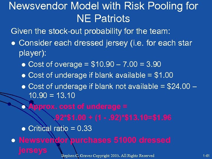Newsvendor Model with Risk Pooling for NE Patriots Given the stock-out probability for the team: l Consider each dressed jersey (i. e. for each star player): Cost of overage = $10. 90 – 7. 00 = 3. 90 l Cost of underage if blank available = $1. 00 l Cost of underage if blank not available = $24. 00 – 10. 90 = 13. 10 l Approx. cost of underage =. 92*$1. 00 + (1 -. 92)*$13. 10=$1. 96 l Critical ratio = 0. 33 l l Newsvendor purchases 51000 dressed jerseys Stephen C. Graves Copyright 2003. All Rights Reserved 1 -61

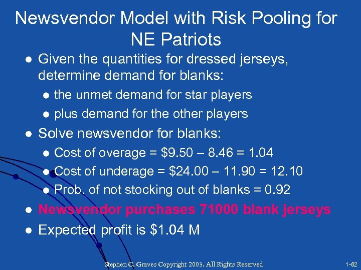Newsvendor Model with Risk Pooling for NE Patriots l Given the quantities for dressed jerseys, determine demand for blanks: the unmet demand for star players l plus demand for the other players l l Solve newsvendor for blanks: Cost of overage = $9. 50 – 8. 46 = 1. 04 l Cost of underage = $24. 00 – 11. 90 = 12. 10 l Prob. of not stocking out of blanks = 0. 92 l l l Newsvendor purchases 71000 blank jerseys Expected profit is $1. 04 M Stephen C. Graves Copyright 2003. All Rights Reserved 1 -62

Results: Newsvendor with Risk Pooling Dressed Blanks Total Purchas e 51227 70932 122159 E[sold] 44265 42712 86976 E[unsold] E[short] 6962 28221 35183 703 Results: Simple Newsvendor Dressed Blanks Total Purchas e 87531 38027 125558 E[sold] 60244 22898 83142 E[unsold] E[short] 27287 15129 42416 Stephen C. Graves Copyright 2003. All Rights Reserved 4161 377 4537 1 -63

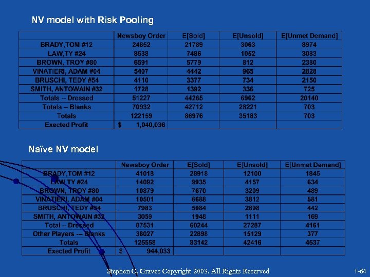NV model with Risk Pooling Naïve NV model Stephen C. Graves Copyright 2003. All Rights Reserved 1 -64

Observations from Example Expected profit increases by 5 to 10% over current practice & naïve newsvendor l Much different solution strategy: blanks used not just for “other” players but also as postponement option l Many more jerseys dressed in Indianapolis l Mix of leftovers is largely blanks l Value of newsvendor perspective l Stephen C. Graves Copyright 2003. All Rights Reserved 1 -65

Outline of Case Discussion Discuss business context, nature of demand, the sales cycle, key success factors, failure modes l Discuss supply chain, planning cycle, planning challenges l Frame as single-season planning problem; relate to newsvendor model l Develop approach and key insights with NE Patriots example l Report on findings for NFL l Wrap up and summary of learnings l Stephen C. Graves Copyright 2003. All Rights Reserved 1 -66

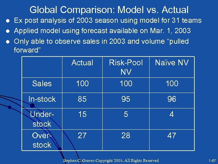Global Comparison: Model vs. Actual l Ex post analysis of 2003 season using model for 31 teams Applied model using forecast available on Mar. 1, 2003 Only able to observe sales in 2003 and volume “pulled forward” Actual Sales 100 Risk-Pool NV 100 Naïve NV In-stock 85 95 96 Understock Overstock 15 5 4 27 28 47 Stephen C. Graves Copyright 2003. All Rights Reserved 100 1 -67

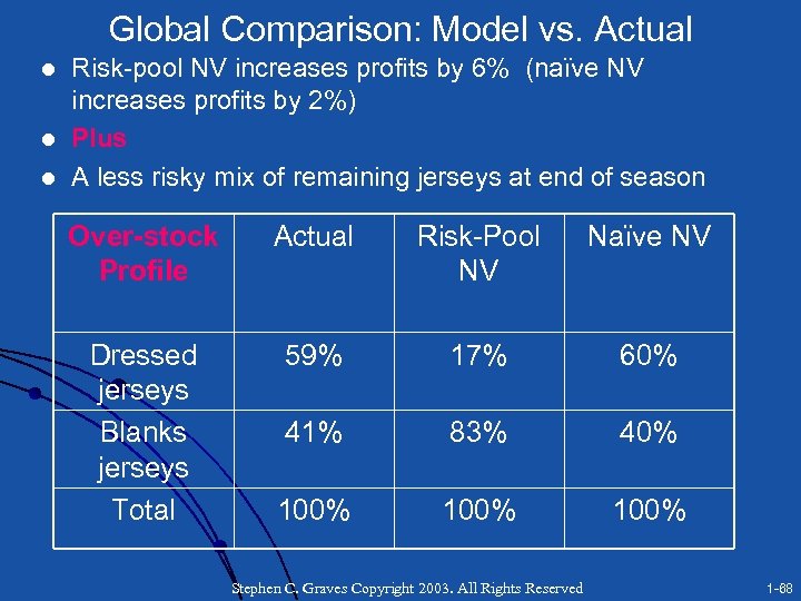Global Comparison: Model vs. Actual l Risk-pool NV increases profits by 6% (naïve NV increases profits by 2%) Plus A less risky mix of remaining jerseys at end of season Over-stock Profile Actual Risk-Pool NV Naïve NV Dressed jerseys Blanks jerseys Total 59% 17% 60% 41% 83% 40% 100% Stephen C. Graves Copyright 2003. All Rights Reserved 1 -68

Outline of Case Discussion l l l Discuss business context, nature of demand, the sales cycle, key success factors, failure modes Discuss supply chain, planning cycle, planning challenges Frame as single-season planning problem; relate to newsvendor model Develop approach and key insights with NE Patriots example Report on findings for NFL Wrap up and summary of learnings Stephen C. Graves Copyright 2003. All Rights Reserved 1 -69

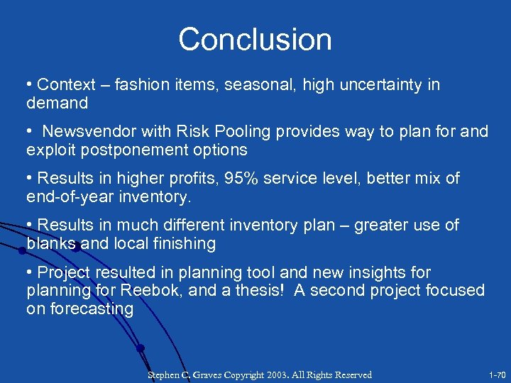Conclusion • Context – fashion items, seasonal, high uncertainty in demand • Newsvendor with Risk Pooling provides way to plan for and exploit postponement options • Results in higher profits, 95% service level, better mix of end-of-year inventory. • Results in much different inventory plan – greater use of blanks and local finishing • Project resulted in planning tool and new insights for planning for Reebok, and a thesis! A second project focused on forecasting Stephen C. Graves Copyright 2003. All Rights Reserved 1 -70