Chapter 5 The Firm And the Isoquant Map

Chapter 5 The Firm And the Isoquant Map

ISOQUANT- ISOCOST ANALYSIS • Isoquant • A line indicating the level of inputs required to produce a given level of output • Iso- meaning - ‘Equal’ – As in ‘Iso’-bars • -’Quant’ as in quantity • Isoquant – a line of equal quantity

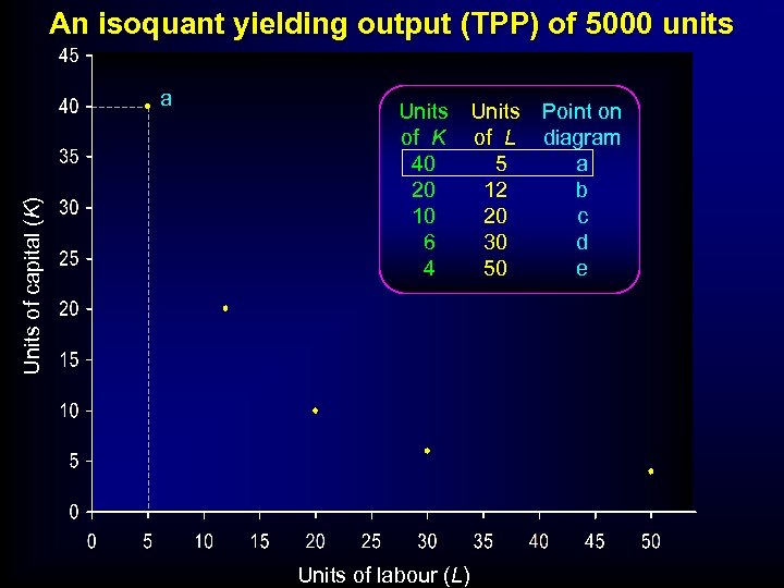An isoquant yielding output (TPP) of 5000 units Units of capital (K) a Units of K 40 20 10 6 4 Units of labour (L) Units of L 5 12 20 30 50 Point on diagram a b c d e

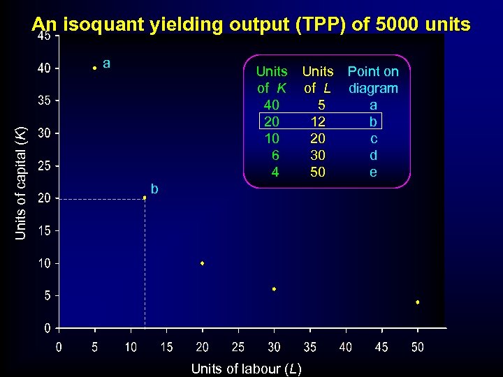An isoquant yielding output (TPP) of 5000 units Units of capital (K) a Units of K 40 20 10 6 4 b Units of labour (L) Units of L 5 12 20 30 50 Point on diagram a b c d e

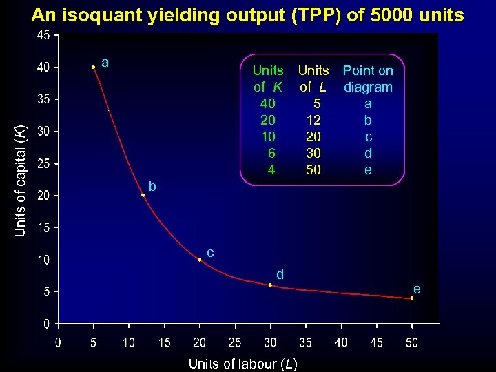An isoquant yielding output (TPP) of 5000 units Units of capital (K) a Units of K 40 20 10 6 4 Units of L 5 12 20 30 50 Point on diagram a b c d e b c d Units of labour (L) e

ISOQUANT- ISOCOST ANALYSIS • Isoquants – their shape – diminishing marginal rate of substitution – Rate at which we can substitute capital for labour and still maintain output at the given level. MRS = DK / DL Sometimes called Marginal rate of Technical Substitution MRTS = DK / DL

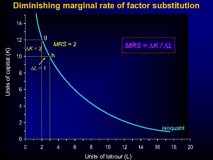Diminishing marginal rate of factor substitution Units of capital (K) g DK = 2 MRS = DK / DL h DL = 1 isoquant Units of labour (L)

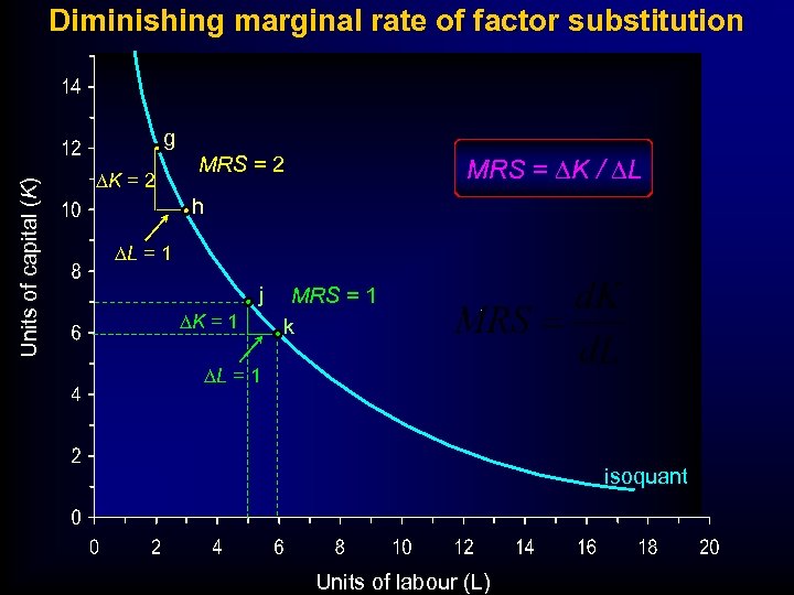Diminishing marginal rate of factor substitution Units of capital (K) g DK = 2 MRS = DK / DL MRS = 2 h DL = 1 j DK = 1 MRS = 1 k DL = 1 isoquant Units of labour (L)

ISOQUANT- ISOCOST ANALYSIS • Isoquants – their shape – diminishing marginal rate of substitution – an isoquant map

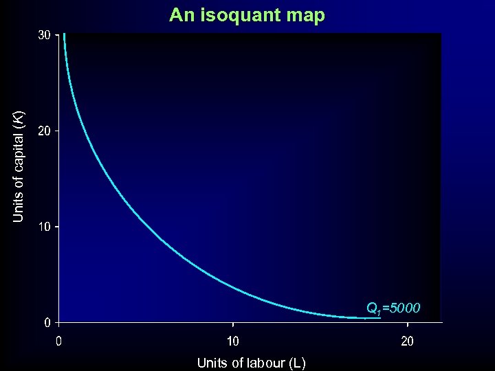Units of capital (K) An isoquant map Q 1=5000 Units of labour (L)

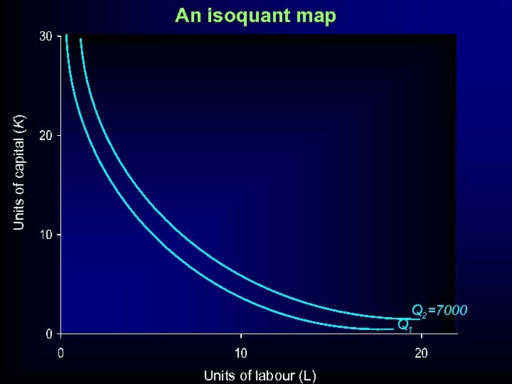Units of capital (K) An isoquant map Q 2=7000 Q 1 Units of labour (L)

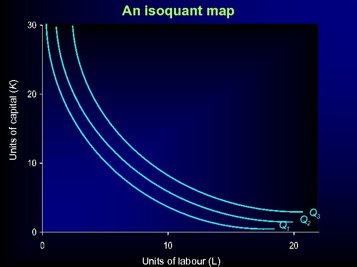Units of capital (K) An isoquant map Q 1 Units of labour (L) Q Q 2 3

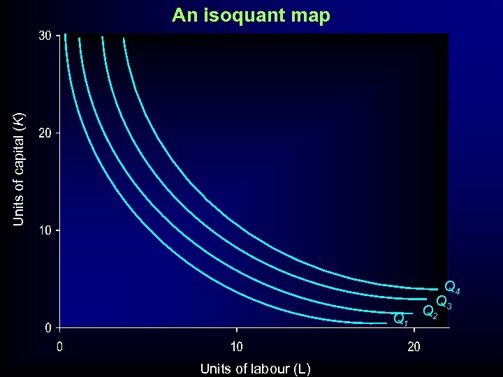Units of capital (K) An isoquant map Q 1 Units of labour (L) Q 4 Q 3 Q 2

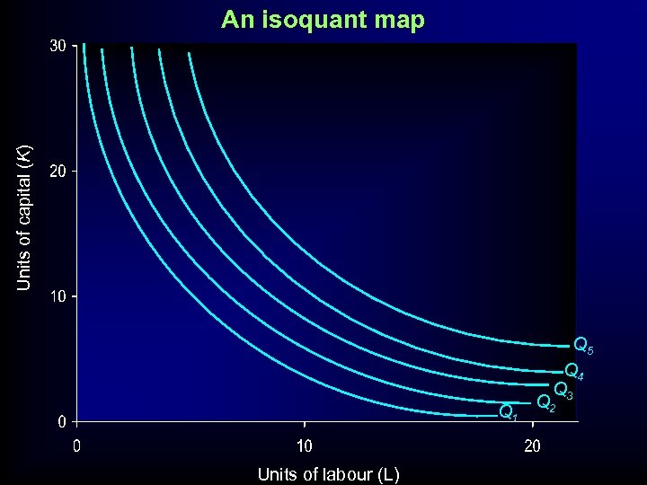Units of capital (K) An isoquant map Q 1 Units of labour (L) Q 5 Q 4 Q 3 Q 2

ISOQUANT- ISOCOST ANALYSIS • Isoquants • E. g: Cobb-Douglas Production Function Q=K 1/2 L 1/2 • Next topic: – isoquants and returns to scale

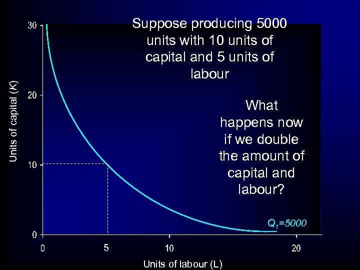Units of capital (K) Suppose producing 5000 units with 10 units of capital and 5 units of labour What happens now if we double the amount of capital and labour? Q 1=5000 5 Units of labour (L)

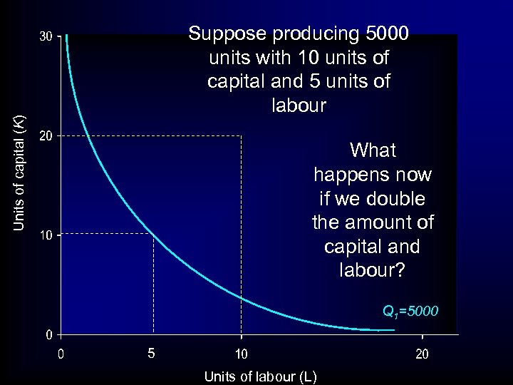Units of capital (K) Suppose producing 5000 units with 10 units of capital and 5 units of labour What happens now if we double the amount of capital and labour? Q 1=5000 5 Units of labour (L)

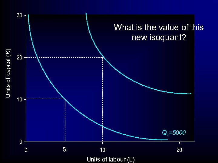Units of capital (K) What is the value of this new isoquant? Q 1=5000 5 Units of labour (L)

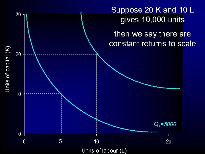Suppose 20 K and 10 L gives 10, 000 units Units of capital (K) then we say there are constant returns to scale Q 1=5000 5 Units of labour (L)

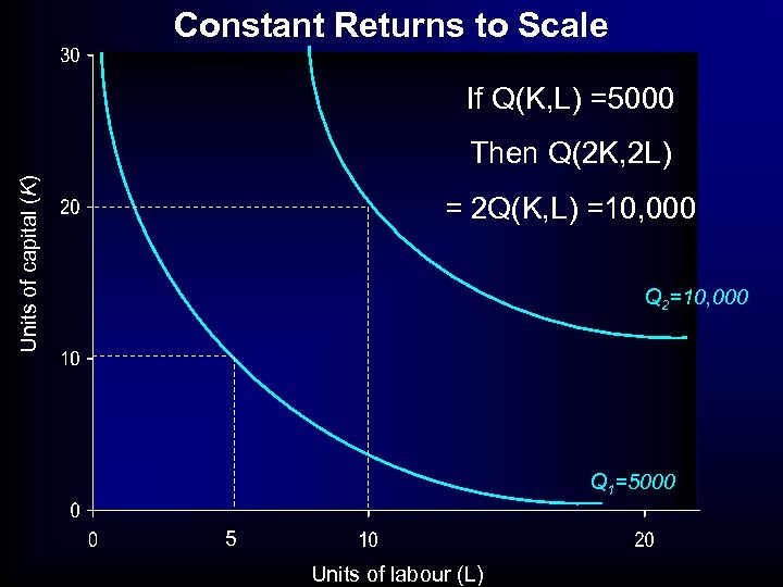Constant Returns to Scale If Q(K, L) =5000 Units of capital (K) Then Q(2 K, 2 L) = 2 Q(K, L) =10, 000 Q 2=10, 000 Q 1=5000 5 Units of labour (L)

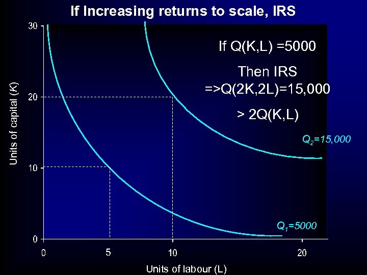If Increasing returns to scale, IRS If Q(K, L) =5000 Units of capital (K) Then IRS =>Q(2 K, 2 L)=15, 000 > 2 Q(K, L) Q 2=15, 000 Q 1=5000 5 Units of labour (L)

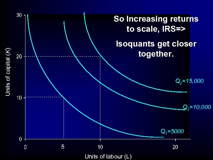So Increasing returns to scale, IRS=> Units of capital (K) Isoquants get closer together. Q 2=15, 000 Q 2=10, 000 Q 1=5000 5 Units of labour (L)

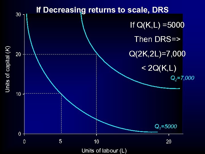If Decreasing returns to scale, DRS If Q(K, L) =5000 Units of capital (K) Then DRS=> Q(2 K, 2 L)=7, 000 < 2 Q(K, L) Q 2=7, 000 Q 1=5000 5 Units of labour (L)

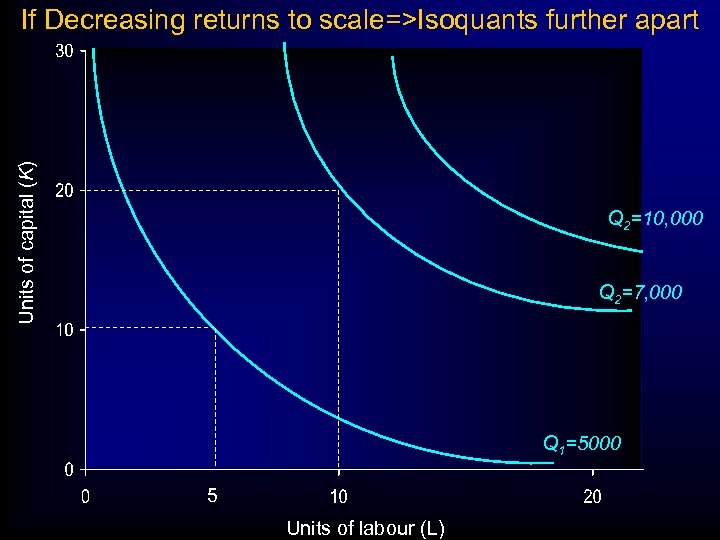Units of capital (K) If Decreasing returns to scale=>Isoquants further apart Q 2=10, 000 Q 2=7, 000 Q 1=5000 5 Units of labour (L)

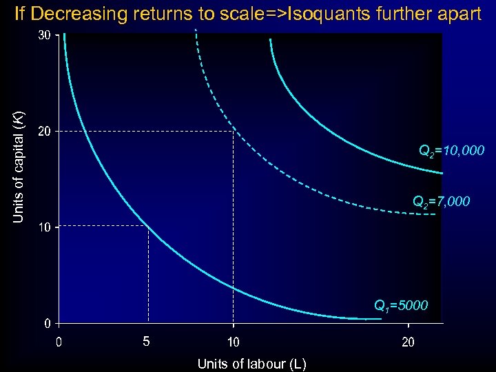Units of capital (K) If Decreasing returns to scale=>Isoquants further apart Q 2=10, 000 Q 2=7, 000 Q 1=5000 5 Units of labour (L)

ISOQUANT- ISOCOST ANALYSIS • Isoquants – their shape – diminishing marginal rate of substitution – isoquants and returns to scale – isoquants and marginal returns

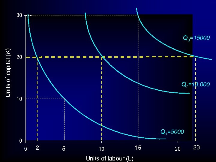
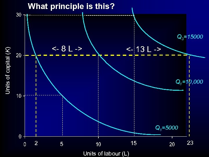
ISOQUANT- ISOCOST ANALYSIS • Isoquants – isoquants and marginal returns: – Marginal Returns means changing one variable and keeping the other constant. – To see this, suppose we examine the CRS diagram again, this time with 3 isoquants, – 5000, 10, 000, and 15, 000

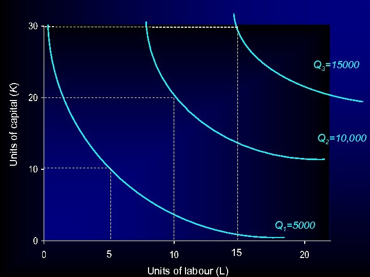Units of capital (K) Q 3=15000 Q 2=10, 000 Q 1=5000 15 5 Units of labour (L)

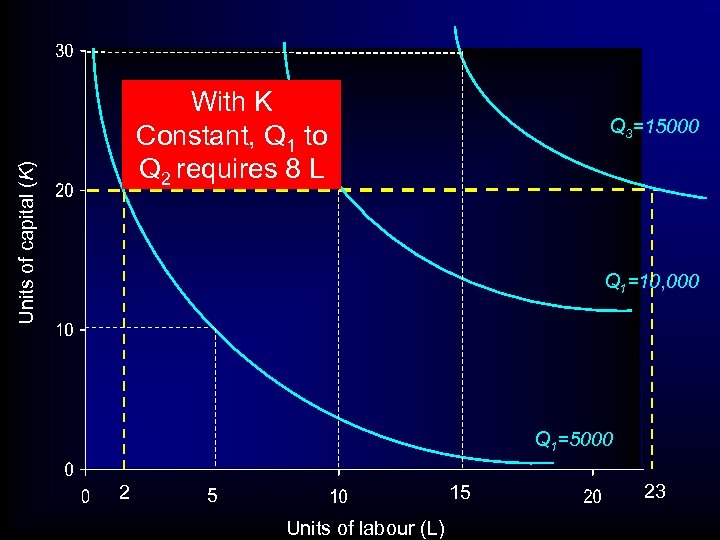
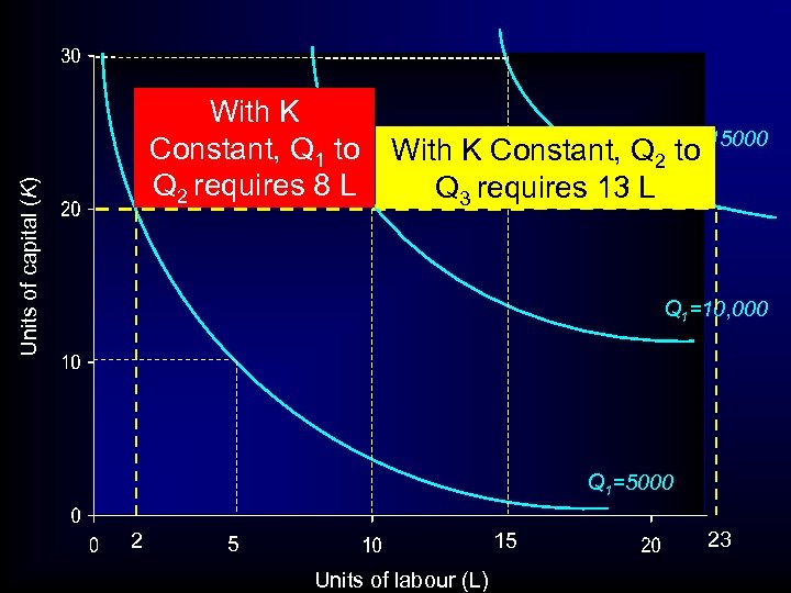
ISOQUANT- ISOCOST ANALYSIS • Next, holding capital constant at K=20 we examine the different amounts of labour required to produce • 5000, 10, 000, and 15, 000 units of output

Units of capital (K) Q 3=15000 Q 1=10, 000 Q 1=5000 2 15 5 Units of labour (L) 23

Units of capital (K) With K Constant, Q 1 to Q 2 requires 8 L Q 3=15000 Q 1=10, 000 Q 1=5000 2 15 5 Units of labour (L) 23

Units of capital (K) With K Constant, Q 1 to Q 2 requires 8 L With K Constant, Q 2 Q 3=15000 to Q 3 requires 13 L Q 1=10, 000 Q 1=5000 2 15 5 Units of labour (L) 23

ISOQUANT- ISOCOST ANALYSIS • So 5000 to 10, 000 requires 8 extra L • 10, 000 to 15, 000 requires 13 extra L

What principle is this? Q 3=15000 Units of capital (K) <- 8 L -> <- 13 L -> Q 1=10, 000 Q 1=5000 2 15 5 Units of labour (L) 23

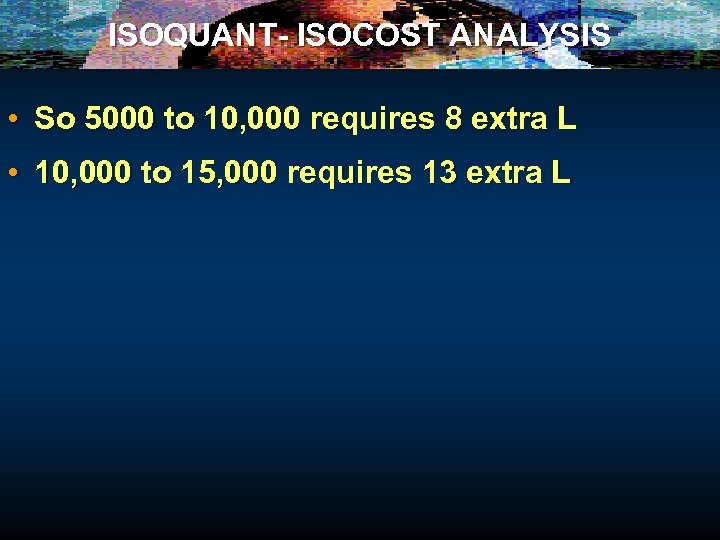
ISOQUANT- ISOCOST ANALYSIS • So 5000 to 10, 000 requires 8 extra L • 10, 000 to 15, 000 requires 13 extra L • What principle is this? • Principle of Diminishing MARGINAL returns • Note can have CRS and diminishing marginal returns

ISOQUANT- ISOCOST ANALYSIS • Isoquants – their shape – diminishing marginal rate of substitution – isoquants and returns to scale – isoquants and marginal returns • Isocosts

ISOQUANT- ISOCOST ANALYSIS • Isoquants – their shape – diminishing marginal rate of substitution – isoquants and returns to scale – isoquants and marginal returns • Isoquants- focussing on issue of efficient way to produce – E. g. Supply Tesco’s with Yogurt

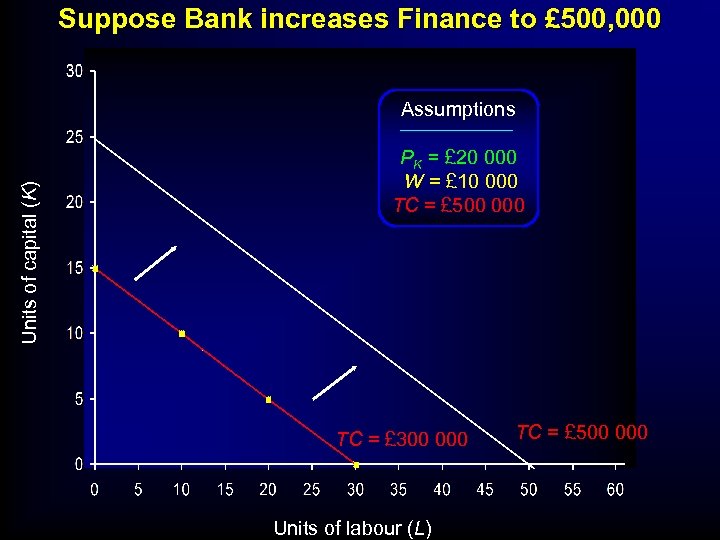
ISOQUANT- ISOCOST ANALYSIS • Other focus might be on Costs: • Suppose bank or venture Capitalist will only lend you £ 300, 000 • What capital and labour will that buy you? • ISOCOST- Line of indicating set of inputs that give ‘equal’ Cost ‘

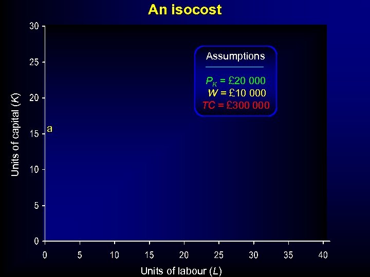An isocost Units of capital (K) Assumptions PK = £ 20 000 W = £ 10 000 TC = £ 300 000 a Units of labour (L)

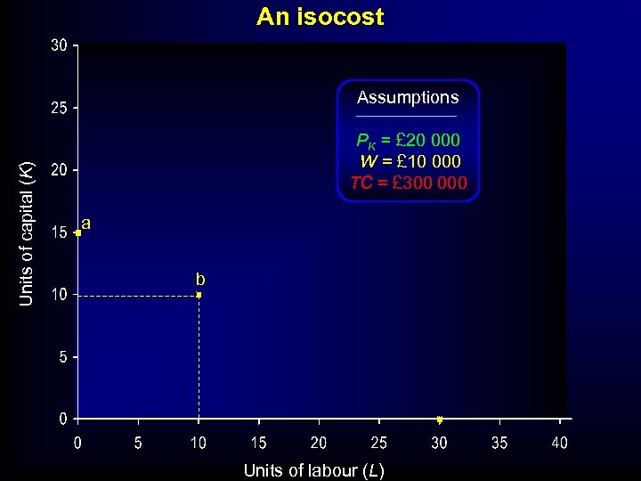An isocost Units of capital (K) Assumptions PK = £ 20 000 W = £ 10 000 TC = £ 300 000 a b Units of labour (L)

An isocost Units of capital (K) Assumptions PK = £ 20 000 W = £ 10 000 TC = £ 300 000 a b c Units of labour (L)

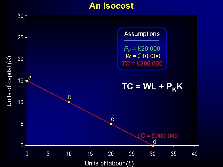An isocost Units of capital (K) Assumptions PK = £ 20 000 W = £ 10 000 TC = £ 300 000 a TC = WL + PKK b c TC = £ 300 000 d Units of labour (L)

ISOQUANT- ISOCOST ANALYSIS • Isoquants – their shape – diminishing marginal rate of substitution – isoquants and returns to scale – isoquants and marginal returns • Isocosts – slope and position of the isocost – shifts in the isocost

Suppose Price of Labour (wages) fell Assumptions Units of capital (K) PK = £ 20 000 W = £ 5, 000 TC = £ 300 000 Slope of Line = -W/PK TC = £ 300 000 Units of labour (L)

Suppose Bank increases Finance to £ 500, 000 Units of capital (K) Assumptions PK = £ 20 000 W = £ 10 000 TC = £ 500 000 TC = £ 300 000 Units of labour (L) TC = £ 500 000

Efficient production: • Effectively have two types of problem • 1. Least-cost combination of factors for a given output • E. g: The supplying Tesco’s problem

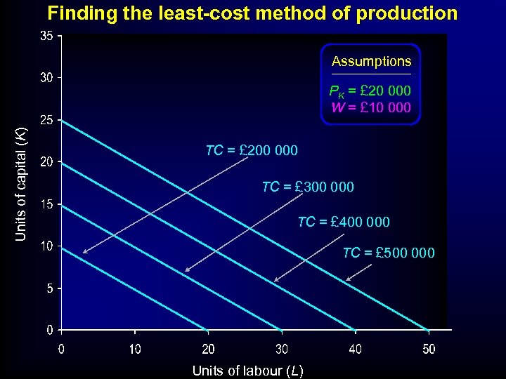Finding the least-cost method of production Assumptions Units of capital (K) PK = £ 20 000 W = £ 10 000 TC = £ 200 000 TC = £ 300 000 TC = £ 400 000 TC = £ 500 000 Units of labour (L)

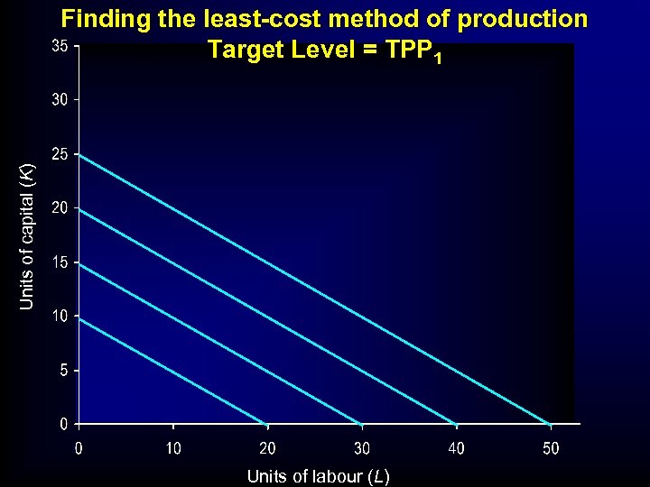Units of capital (K) Finding the least-cost method of production Target Level = TPP 1 Units of labour (L)

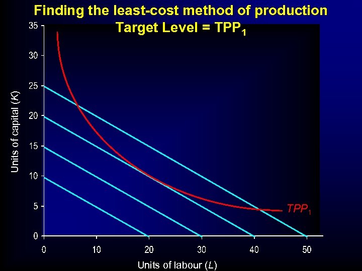Units of capital (K) Finding the least-cost method of production Target Level = TPP 1 Units of labour (L)

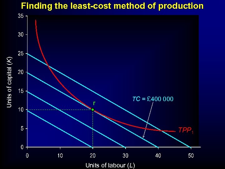Units of capital (K) Finding the least-cost method of production r TC = £ 400 000 TPP 1 Units of labour (L)

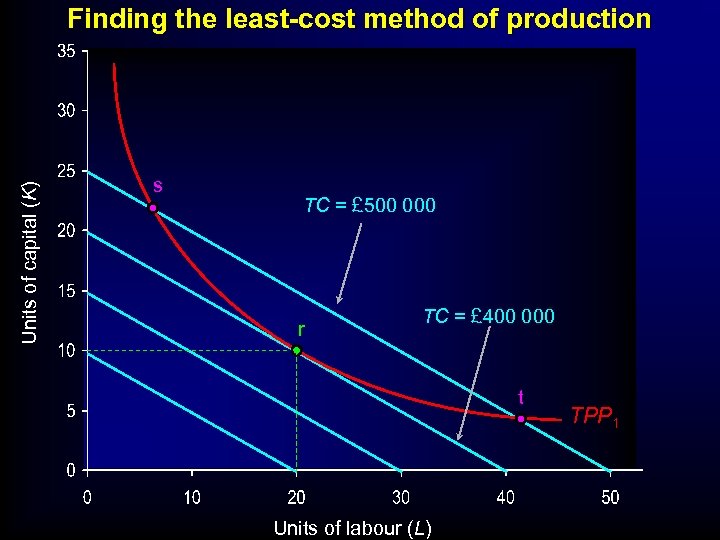Units of capital (K) Finding the least-cost method of production s TC = £ 500 000 r TC = £ 400 000 t Units of labour (L) TPP 1

ISOQUANT- ISOCOST ANALYSIS • Least-cost combination of factors for a given output – Produce on lowest isocost line where the iosquant just touches it at a point of tangency

ISOQUANT- ISOCOST ANALYSIS • Least-cost combination of factors for a given output – point of tangency – comparison with marginal productivity approach • Marginal Productivity Approach

Efficient production: • Effectively have two types of problem • 1. Least-cost combination of factors for a given output • 2. Highest output for a given cost of production • . Here have Financial Constraint: • . E. g. : Venture Capital

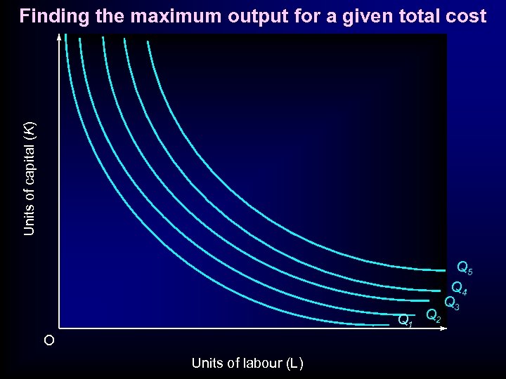Units of capital (K) Finding the maximum output for a given total cost Q 1 Q 2 O Units of labour (L) Q 5 Q 4 Q 3

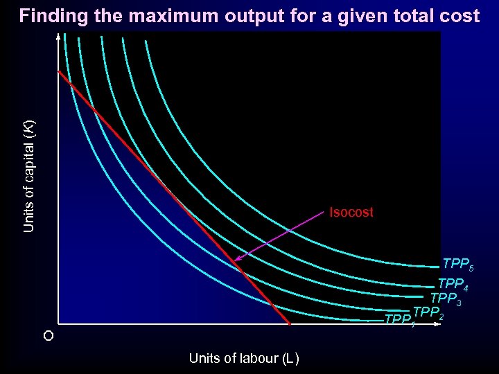Units of capital (K) Finding the maximum output for a given total cost Isocost TPP 5 TPP 4 TPP 3 TPP 2 TPP 1 O Units of labour (L)

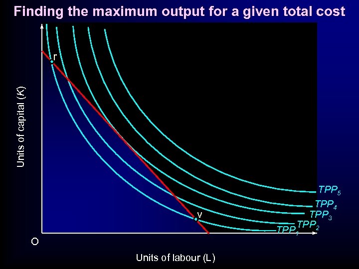Finding the maximum output for a given total cost Units of capital (K) r v TPP 5 TPP 4 TPP 3 TPP 2 TPP 1 O Units of labour (L)

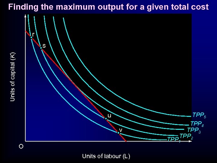Finding the maximum output for a given total cost r Units of capital (K) s u v TPP 5 TPP 4 TPP 3 TPP 2 TPP 1 O Units of labour (L)

Finding the maximum output for a given total cost r Units of capital (K) s t u v TPP 5 TPP 4 TPP 3 TPP 2 TPP 1 O Units of labour (L)

Finding the maximum output for a given total cost r Units of capital (K) s K 1 t u v O TPP 5 TPP 4 TPP 3 TPP 2 TPP 1 L 1 Units of labour (L)

Efficient production: • Effectively have two types of problem • 1. Least-cost combination of factors for a given output • 2. Highest output for a given cost of production • Comparison with Marginal Product Approach

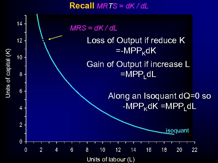Recall MRTS = d. K / d. L Units of capital (K) MRS = d. K / d. L Loss of Output if reduce K =-MPPKd. K Gain of Output if increase L =MPPLd. L Along an Isoquant d. Q=0 so -MPPKd. K =MPPLd. L isoquant Units of labour (L)

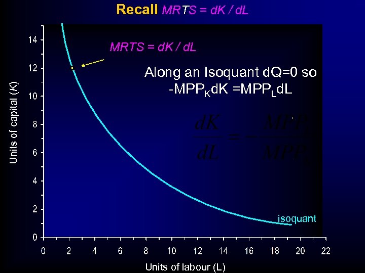Recall MRTS = d. K / d. L Units of capital (K) MRTS = d. K / d. L Along an Isoquant d. Q=0 so -MPPKd. K =MPPLd. L isoquant Units of labour (L)

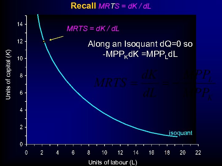Recall MRTS = d. K / d. L Units of capital (K) MRTS = d. K / d. L Along an Isoquant d. Q=0 so -MPPKd. K =MPPLd. L isoquant Units of labour (L)

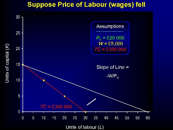
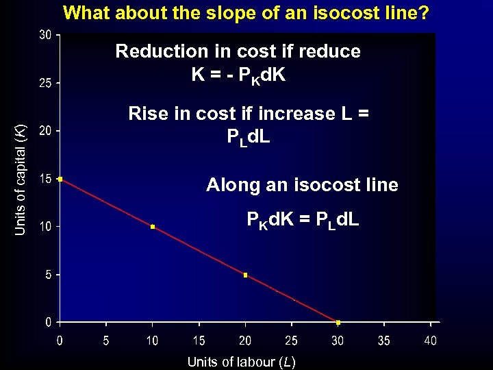What about the slope of an isocost line? Units of capital (K) Reduction in cost if reduce K = - PKd. K Rise in cost if increase L = PLd. L Along an isocost line PKd. K = PLd. L Units of labour (L)

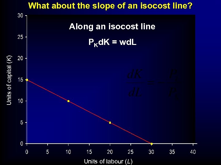What about the slope of an isocost line? Along an isocost line Units of capital (K) PKd. K = wd. L Units of labour (L)

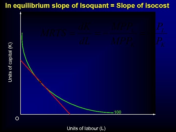Units of capital (K) In equilibrium slope of Isoquant = Slope of isocost 100 O Units of labour (L)

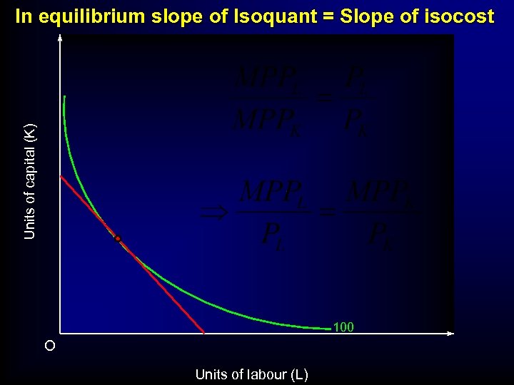Units of capital (K) In equilibrium slope of Isoquant = Slope of isocost 100 O Units of labour (L)

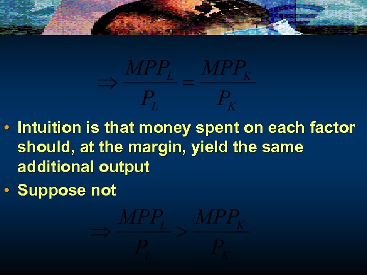• Intuition is that money spent on each factor should, at the margin, yield the same additional output • Suppose not

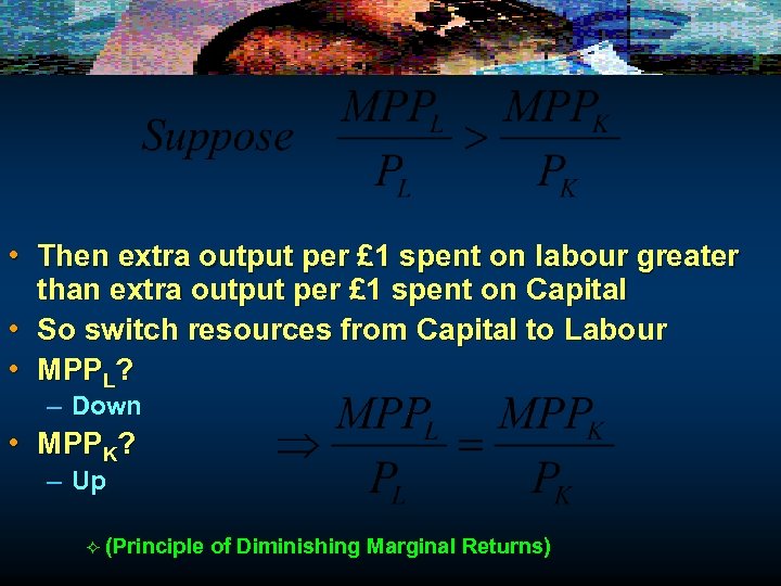• Then extra output per £ 1 spent on labour greater than extra output per £ 1 spent on Capital • So switch resources from Capital to Labour • MPPL? – Down • MPPK? – Up ² (Principle of Diminishing Marginal Returns)

LONG-RUN COSTS • Derivation of long-run costs from an isoquant map – derivation of long-run costs

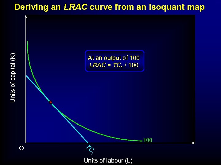Units of capital (K) Deriving an LRAC curve from an isoquant map At an output of 100 LRAC = TC 1 / 100 TC O 1 Units of labour (L)

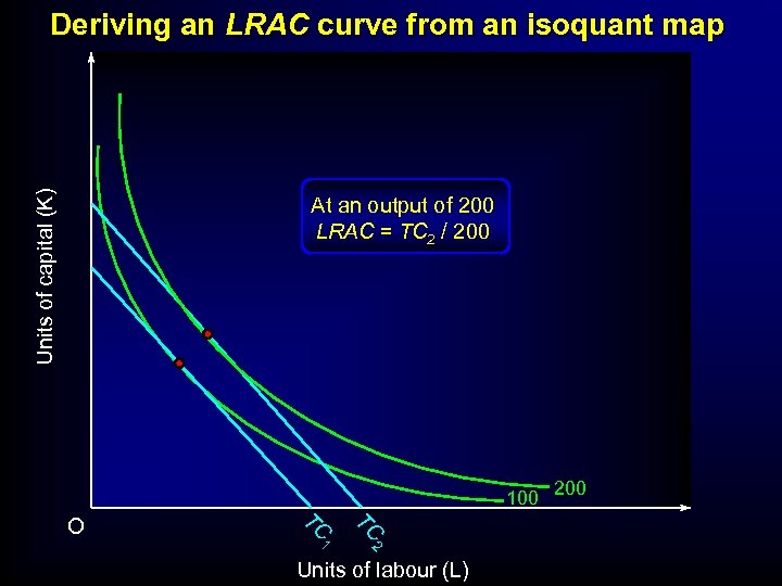Units of capital (K) Deriving an LRAC curve from an isoquant map At an output of 200 LRAC = TC 2 / 200 100 200 TC TC 1 2 O Units of labour (L)

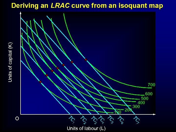Units of capital (K) Deriving an LRAC curve from an isoquant map 700 100 200 TC TC 5 6 7 Units of labour (L) TC 2 4 TC 1 TC 3 TC TC O 600 500 400 300

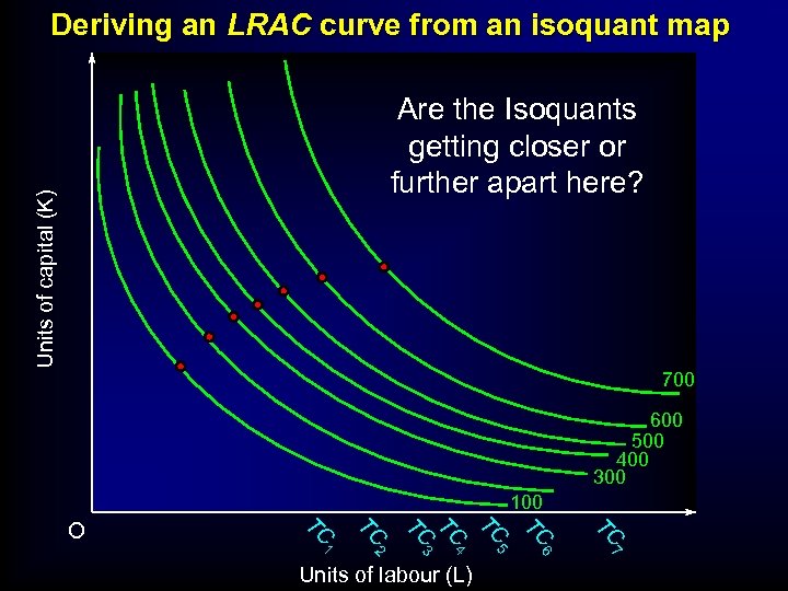Deriving an LRAC curve from an isoquant map Units of capital (K) Are the Isoquants getting closer or further apart here? 700 600 500 400 300 100 TC TC 5 6 7 Units of labour (L) TC 2 4 TC 1 TC 3 TC TC O

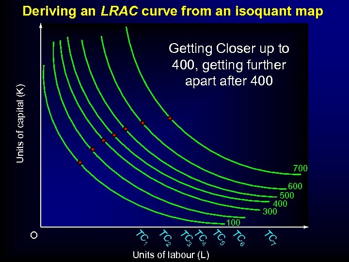Deriving an LRAC curve from an isoquant map Units of capital (K) Getting Closer up to 400, getting further apart after 400 700 600 500 400 300 100 TC TC 5 6 7 Units of labour (L) TC 2 4 TC 1 TC 3 TC TC O

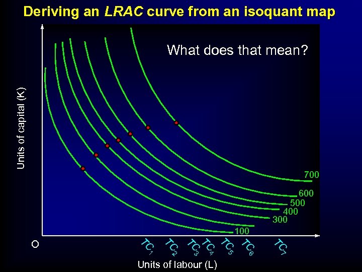Deriving an LRAC curve from an isoquant map Units of capital (K) What does that mean? 700 600 500 400 300 100 TC TC 5 6 7 Units of labour (L) TC 2 4 TC 1 TC 3 TC TC O

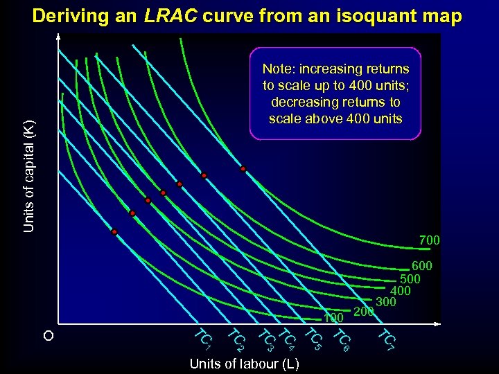Deriving an LRAC curve from an isoquant map Units of capital (K) Note: increasing returns to scale up to 400 units; decreasing returns to scale above 400 units 700 100 200 TC TC 5 6 7 Units of labour (L) TC 2 4 TC 1 TC 3 TC TC O 600 500 400 300

LONG-RUN COSTS • Derivation of long-run costs from an isoquant map – derivation of long-run costs – the expansion path

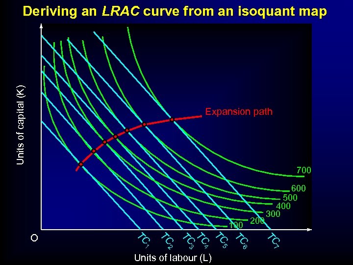Units of capital (K) Deriving an LRAC curve from an isoquant map Expansion path 700 100 200 TC TC 5 6 7 Units of labour (L) TC 2 4 TC 1 TC 3 TC TC O 600 500 400 300

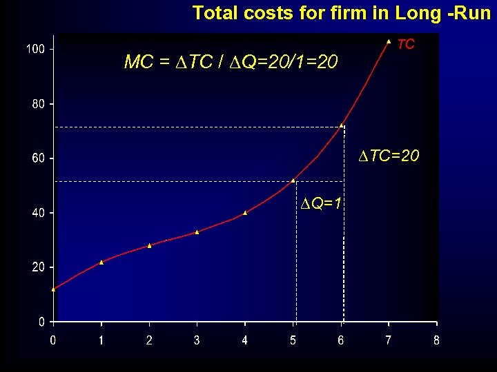Total costs for firm in Long -Run MC = DTC / DQ=20/1=20 TC DTC=20 DQ=1

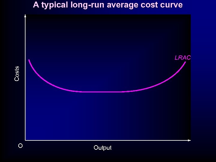A typical long-run average cost curve Costs LRAC O Output

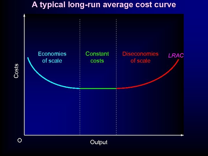Costs A typical long-run average cost curve O Economies of scale Constant costs Output Diseconomies of scale LRAC

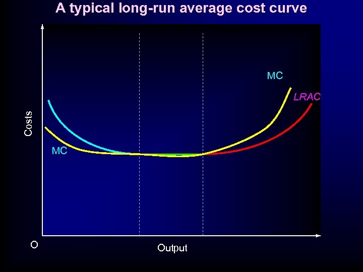A typical long-run average cost curve MC Costs LRAC MC O Output

What about the Short-Run • Derivation of short-run costs from an isoquant map – Recall in SR Capital stock is fixed

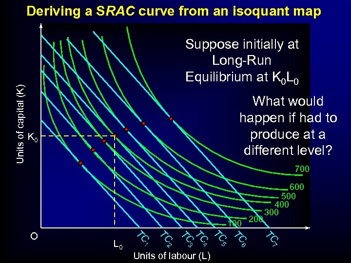Units of capital (K) Deriving a SRAC curve from an isoquant map Suppose initially at Long-Run Equilibrium at K 0 L 0 What would happen if had to produce at a different level? K 0 700 100 200 TC TC 5 6 7 Units of labour (L) TC 4 2 TC 3 TC TC 1 L 0 TC O 600 500 400 300

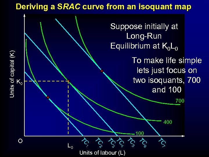Units of capital (K) Deriving a SRAC curve from an isoquant map Suppose initially at Long-Run Equilibrium at K 0 L 0 To make life simple lets just focus on two isoquants, 700 and 100 K 0 700 400 100 TC TC 5 6 7 Units of labour (L) TC 4 2 TC 3 TC TC 1 L 0 TC O

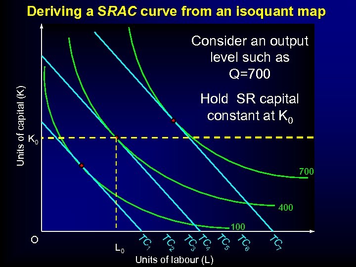Deriving a SRAC curve from an isoquant map Units of capital (K) Consider an output level such as Q=700 Hold SR capital constant at K 0 700 400 100 TC TC 5 6 7 Units of labour (L) TC 4 2 TC 3 TC TC 1 L 0 TC O

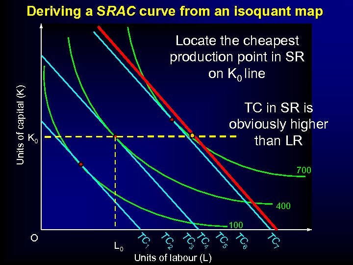Deriving a SRAC curve from an isoquant map Units of capital (K) Locate the cheapest production point in SR on K 0 line TC in SR is obviously higher than LR K 0 700 400 100 TC TC 5 6 7 Units of labour (L) TC 4 2 TC 3 TC TC 1 L 0 TC O

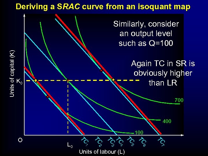Deriving a SRAC curve from an isoquant map Units of capital (K) Similarly, consider an output level such as Q=100 Again TC in SR is obviously higher than LR K 0 700 400 100 TC TC 5 6 7 Units of labour (L) TC 4 2 TC 3 TC TC 1 L 0 TC O

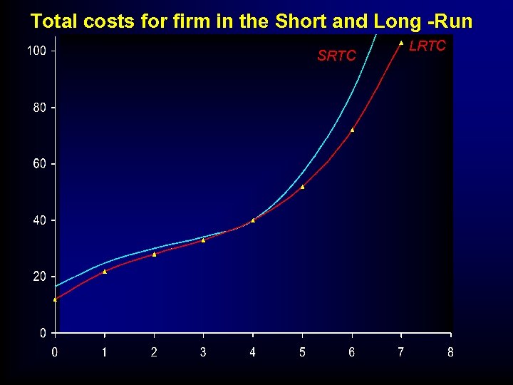Total costs for firm in the Short and Long -Run SRTC LRTC

What about the Short-Run • Derivation of short-run costs from an isoquant map – Recall in SR Capital stock is fixed • In SR TC is always higher than LR • …. and Average costs?

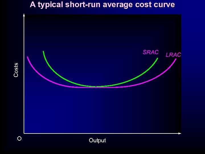A typical short-run average cost curve Costs SRAC O Output LRAC

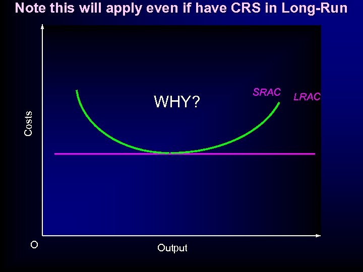Note this will apply even if have CRS in Long-Run Costs WHY? O Output SRAC LRAC

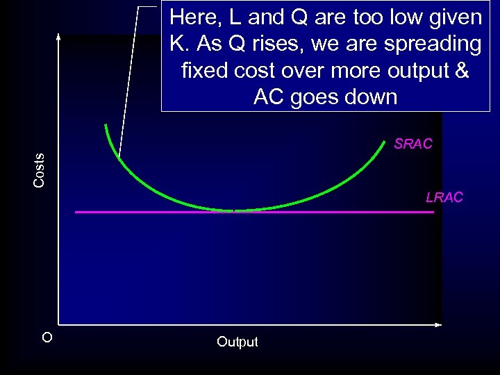Here, L and Q are too low given K. As Q rises, we are spreading fixed cost over more output & AC goes down Costs SRAC LRAC O Output

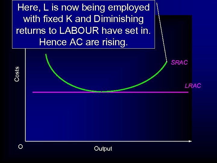Here, L is now being employed with fixed K and Diminishing returns to LABOUR have set in. Hence AC are rising. Costs SRAC LRAC O Output

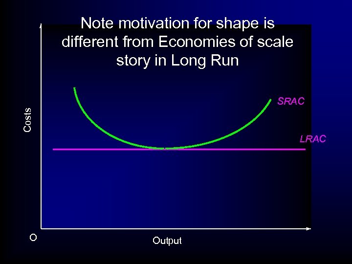Note motivation for shape is different from Economies of scale story in Long Run Costs SRAC LRAC O Output