Chapter 5 Schema Matching and Mapping PRINCIPLES OF

Chapter 5: Schema Matching and Mapping PRINCIPLES OF DATA INTEGRATION ANHAI DOAN ALON HALEVY ZACHARY IVES

Introduction § We have described § formalisms to specify source descriptions § algorithms that use these descriptions to reformulate queries § How to create the source descriptions? § often begin by creating semantic matches v name = title, location = concat(city, state, zipcode) § then elaborate matches into semantic mappings v e. g. , structured queries in a language such as SQL § Schema matching and mapping are often quite difficult § This chapter describes matching and mapping tools § that can significantly reduce the time it takes for the developer to create matches and mappings 2

Outline § Problem definition, challenges, and overview § Schema matching § § § Matchers Combining match predictions Enforcing domain integrity constraints Match selector Reusing previous matches Many-to-many matches § Schema mapping 3

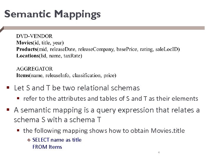Semantic Mappings § Let S and T be two relational schemas § refer to the attributes and tables of S and T as their elements § A semantic mapping is a query expression that relates a schema S with a schema T § the following mapping shows how to obtain Movies. title v SELECT name as title FROM Items 4

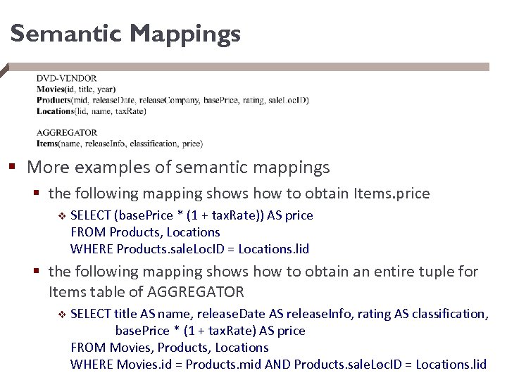Semantic Mappings § More examples of semantic mappings § the following mapping shows how to obtain Items. price v SELECT (base. Price * (1 + tax. Rate)) AS price FROM Products, Locations WHERE Products. sale. Loc. ID = Locations. lid § the following mapping shows how to obtain an entire tuple for Items table of AGGREGATOR v SELECT title AS name, release. Date AS release. Info, rating AS classification, base. Price * (1 + tax. Rate) AS price FROM Movies, Products, Locations 5 WHERE Movies. id = Products. mid AND Products. sale. Loc. ID = Locations. lid

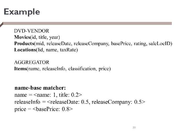
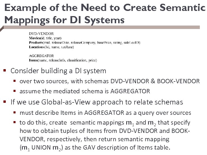Example of the Need to Create Semantic Mappings for DI Systems § Consider building a DI system § over two sources, with schemas DVD-VENDOR & BOOK-VENDOR § assume the mediated schema is AGGREGATOR § If we use Global-as-View approach to relate schemas § must describe Items in AGGREGATOR as a query over sources § to do this, create semantic mappings m 1 and m 2 that specify how to obtain tuples of Items from DVD-VENDOR and BOOKVENDOR, respectively, then return semantic mapping (m 1 UNION m 2) as the GAV description of Items table. 6

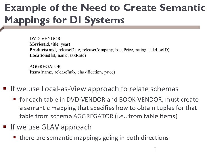Example of the Need to Create Semantic Mappings for DI Systems § If we use Local-as-View approach to relate schemas § for each table in DVD-VENDOR and BOOK-VENDOR, must create a semantic mapping that specifies how to obtain tuples for that table from schema AGGREGATOR (i. e. , from table Items) § If we use GLAV approach § there are semantic mappings going in both directions 7

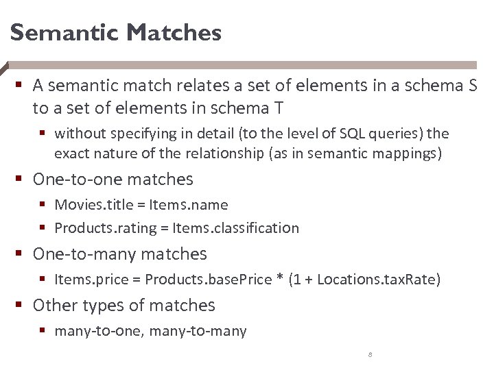Semantic Matches § A semantic match relates a set of elements in a schema S to a set of elements in schema T § without specifying in detail (to the level of SQL queries) the exact nature of the relationship (as in semantic mappings) § One-to-one matches § Movies. title = Items. name § Products. rating = Items. classification § One-to-many matches § Items. price = Products. base. Price * (1 + Locations. tax. Rate) § Other types of matches § many-to-one, many-to-many 8

Relationship between Schema Matching and Mapping § To create source description § often start by creating semantic matches § then elaborate matches into mappings § Why start with semantic matches? § they are often easier to elicit from designers v e. g. , can specify price = base. Price * (1 + tax. Rate) from domain knowledge § Why the need to elaborate matches into mappings? § § matches often specify functional relationships but they cannot be used to obtain data instances need SQL queries, that is, mappings for that purpose so matches need to be elaborated into mappings 9

Relationship between Schema Matching and Mapping § Example: elaborate the match § price = base. Price * (1 + tax. Rate) into mapping § SELECT (base. Price * (1 + tax. Rate)) AS price FROM Product, Location WHERE Product. sale. Loc. ID = Location. lid § Another reason for starting with matches § break the long process in the middle § allow designer to verify and correct the matches § thus reducing the complexity of the overall process 10

Challenges of Schema Matching and Mapping § Matching and mapping systems must reconcile semantic heterogeneity between the schemas § Such semantic heterogeneity arise in many ways § same concept, but different names for tables and attributes v rating vs classification § multiple attributes in 1 schema relate to 1 attribute in the other v base. Price and tax. Rate relate to price § tabular organization of schemas can be quite different v one table in AGGREGATOR vs three tables in DVD-VENDOR § coverage and level of details can also differ significantly v DVD-VENDOR also models release. Date and release. Company 11

Challenges of Schema Matching and Mapping § Why do we have semantic heterogeneity? § schemas are created by different people whose states and styles are different § disparate databases are rarely created for exact same purposes § Why reconciling semantic heterogeneity is hard § § the semantics is not fully captured in the schemas schema clues can be unreliable intended semantics can be subjective correctly combining the data is difficult § Standard is not a solution! § works for limited use cases where number of attributes is small and there is strong incentive to agree on them 12

Overview of Matching Systems § For now we consider only 1 -1 matching systems § will discuss finding complex matches later § Key observation: need multiple heuristics / types of information to maximize matching accuracy § e. g. , by matching the names, can infer that release. Info = release. Date or release. Info = release. Company, but do not know which one § by matching the data values, can infer that release. Info = release. Date or release. Info = year, but do not know which one § by combining both, can infer that release. Info = release. Date 13

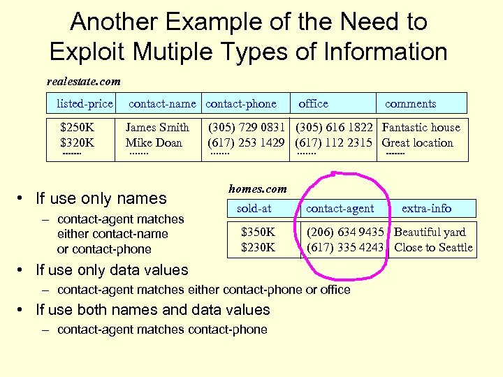Another Example of the Need to Exploit Mutiple Types of Information realestate. com listed-price contact-name contact-phone $250 K $320 K James Smith Mike Doan • If use only names – contact-agent matches either contact-name or contact-phone office comments (305) 729 0831 (305) 616 1822 Fantastic house (617) 253 1429 (617) 112 2315 Great location homes. com sold-at $350 K $230 K contact-agent (206) 634 9435 Beautiful yard (617) 335 4243 Close to Seattle • If use only data values – contact-agent matches either contact-phone or office • If use both names and data values – contact-agent matches contact-phone extra-info

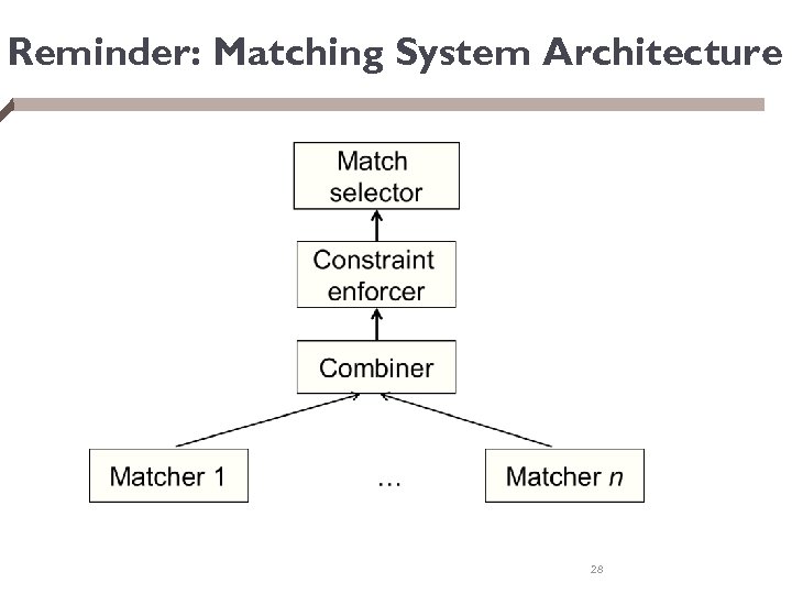
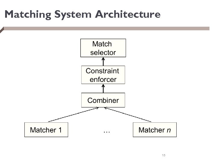Matching System Architecture 15

Overview of Mapping Systems § Input: matches, output: actual mappings § Key challenge: find how tuples from one source can be transformed and combined to produce tuples in the other § which data transformation to apply? § which joins to take? § and many more possible decisions 16

Outline § Problem definition, challenges, and overview § Schema matching § § § Matchers Combining match predictions Enforcing domain integrity constraints Match selector Reusing previous matches Many-to-many matches § Schema mapping 17

Matchers § schemas similarity matrix § Input: two schemas S and T, plus any possibly helpful auxiliary information (e. g. , data instances, text descriptions) § Output: sim matrix that assigns to each element pair of S and T a number in [0, 1] predicting whether the pair match § Numerous matchers have been proposed § We describe a few, in two classes: name matchers and data matchers 18

Name-Based Matchers § Use string matching techniques § e. g. , edit distance, Jaccard, Soundex, etc. § Often have to pre-process names § split them using certain delimiters v e. g. , sale. Loc. ID sale, Loc, ID § expand known abbreviations or acronyms v location, customer § expand a string with synonyms / hypernyms v add cost to price, expand product into book, dvd, cd § remove stop words v in, at, and 19

Example 20

Instance-Based Matchers § When schemas come with data instances, these can be extremely helpful in deciding matches § Many instance-based matchers have been proposed § Some of the most popular § recognizers v use dictionaries, regexes, or simple rules § overlap matchers v examine the overlap of values among attributes § classifiers v use learning techniques 21

Building Recognizers § Use dictionaries, regexes, or rules to recognize data values of certain kinds of attributes § Example attributes for which recognizers are well suited § § country names, city names, US states person names (can use dictionaries of last and first names) color, rating (e. g. , G, PG-13, etc. ), phone, fax, soc sec genes, protein, zip codes 22

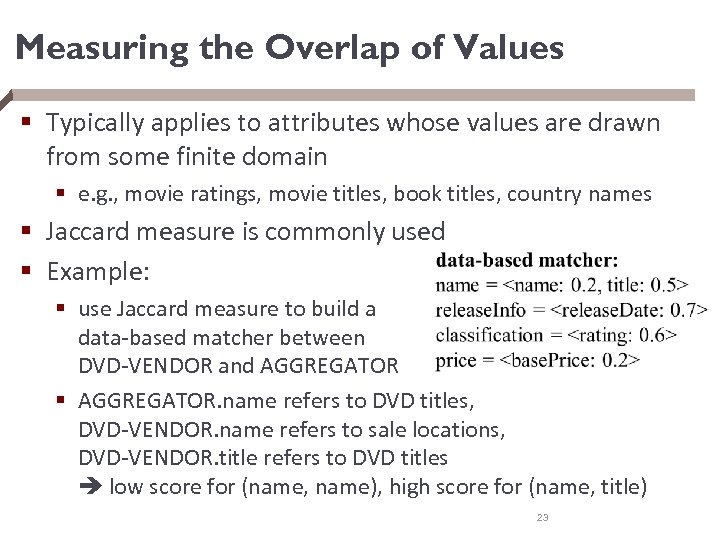Measuring the Overlap of Values § Typically applies to attributes whose values are drawn from some finite domain § e. g. , movie ratings, movie titles, book titles, country names § Jaccard measure is commonly used § Example: § use Jaccard measure to build a data-based matcher between DVD-VENDOR and AGGREGATOR § AGGREGATOR. name refers to DVD titles, DVD-VENDOR. name refers to sale locations, DVD-VENDOR. title refers to DVD titles low score for (name, name), high score for (name, title) 23

Using Classifiers § Builds classifiers on one schema and uses them to classify the elements of the other schema § e. g. , use Naïve Bayes, decision tree, rule learning, SVM § A common strategy § for each element si of schema S, want to train classifier Ci to recognizer instances of si § to do this, need positive and negative training examples take all data instances of si (that are available) to be positive examples v take all data instances of other elements of S to be negative examples v § train Ci on the positive and negative examples 24

Using Classifiers § A common strategy (cont. ) § now we can use Ci to compute sim score between si and each element tj of schema T § to do this, apply Ci to data instances of tj v for each instance, Ci produces a number in [0, 1] that is the confidence that the instance is indeed an instance of si § now need to aggregate the confidence scores of the instances (of tj) to return a single confidence score (as the sim score between si and tj) § a simple way to do so is to compute the average score over all instances of tj 25

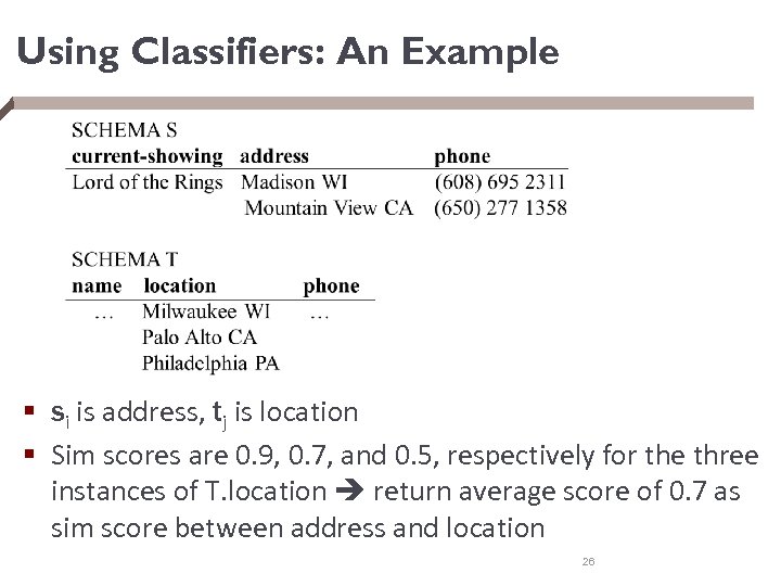Using Classifiers: An Example § si is address, tj is location § Sim scores are 0. 9, 0. 7, and 0. 5, respectively for the three instances of T. location return average score of 0. 7 as sim score between address and location 26

Using Classifiers § Designer decides which schema should play the role of schema S (on which to build classifiers) § typically chooses the mediated schema to be S, so that can reuse the classifiers to match the schemas of new data sources § May want to do it both ways § build classifiers on S and use them to classify instances of T § then build classifiers on T and use them to classify instances of S § e. g. , when both S and T are taxonomies of concepts v see the bibliographic notes 27

Reminder: Matching System Architecture 28

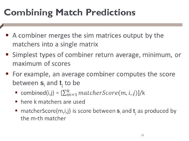Combining Match Predictions § 29

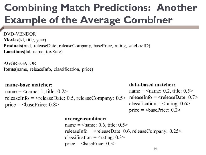Combining Match Predictions: Another Example of the Average Combiner 30

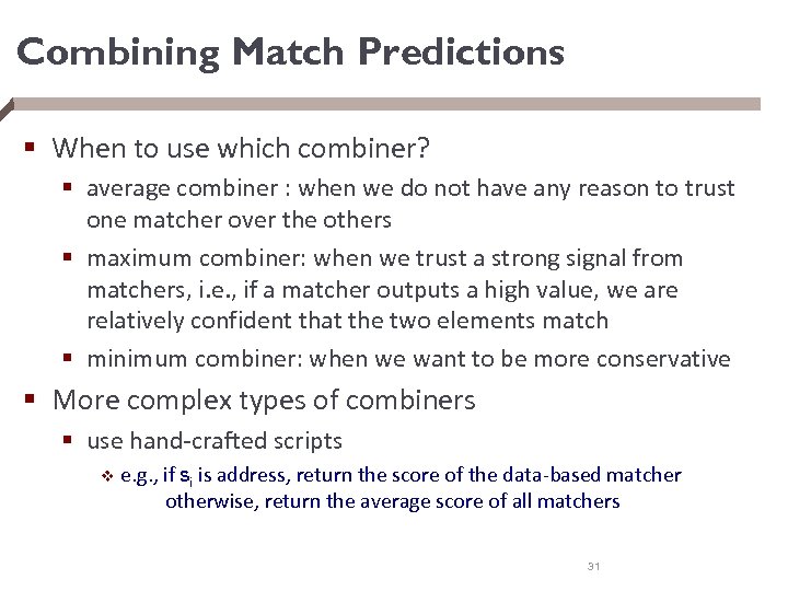Combining Match Predictions § When to use which combiner? § average combiner : when we do not have any reason to trust one matcher over the others § maximum combiner: when we trust a strong signal from matchers, i. e. , if a matcher outputs a high value, we are relatively confident that the two elements match § minimum combiner: when we want to be more conservative § More complex types of combiners § use hand-crafted scripts v e. g. , if si is address, return the score of the data-based matcher otherwise, return the average score of all matchers 31

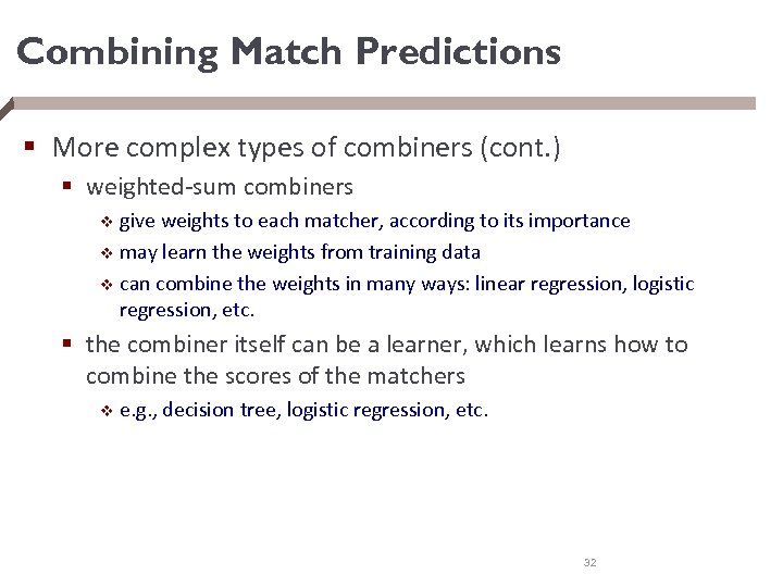Combining Match Predictions § More complex types of combiners (cont. ) § weighted-sum combiners give weights to each matcher, according to its importance v may learn the weights from training data v can combine the weights in many ways: linear regression, logistic regression, etc. v § the combiner itself can be a learner, which learns how to combine the scores of the matchers v e. g. , decision tree, logistic regression, etc. 32

Reminder: Matching System Architecture 33

Enforcing Domain Integrity Constraints § Designer often has knowledge that can be naturally expressed as domain integrity constraints § Constraint enforcer exploits these to prune certain match combinations § searches through the space of all match combinations produced by the combiner § finds one combination with the highest aggregated confidence score that satisfies the constraints 34

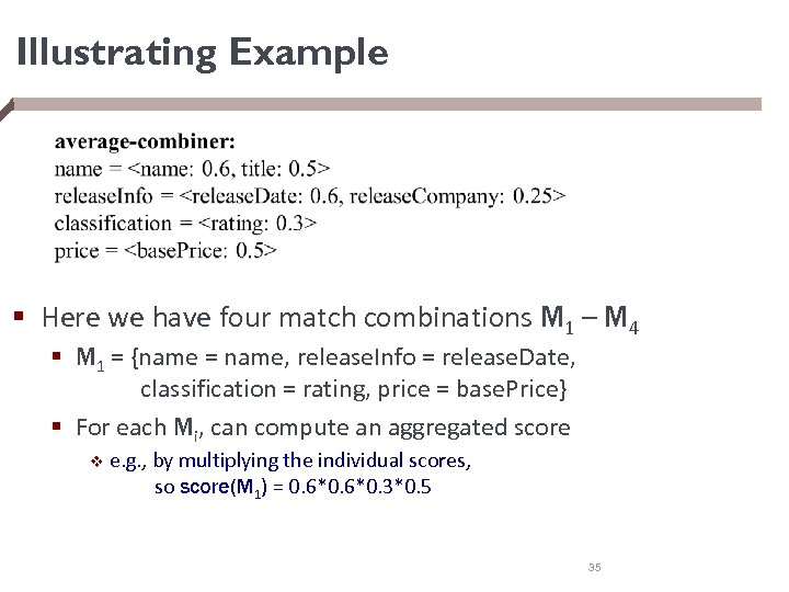Illustrating Example § Here we have four match combinations M 1 – M 4 § M 1 = {name = name, release. Info = release. Date, classification = rating, price = base. Price} § For each Mi, can compute an aggregated score v e. g. , by multiplying the individual scores, so score(M 1) = 0. 6*0. 3*0. 5 35

Illustrating Example (Cont. ) § Suppose designer knows that § AGGREGATOR. name refers to movie titles § many movie titles contain at least four words § Designer can specify a constraint such as § if an attribute A matches AGGREGATOR. name, then in any random sample of 100 data values of A, at least 10 values must contain four words or more § Now the constraint enforcer can search for the best match combination that satisfies this constraint 36

Illustrating Example (Cont. ) § How to search? § conceptually, check the combination with the highest score, M 1: it does not satisfy the constraint § check the combination with the next highest score, M 2: this one satisfies the constraint, so return it as the desired match combination v name = title, release. Info = release. Date, classification = rating, price = base. Price § In practice exploiting constraints is quite hard § must handle a variety of constraints § must find a way to search efficiently 37

Domain Integrity Constraints § Two kinds of constraints: hard and soft § Hard constraints § must be enforced § no output match combination can violate them § Soft constraints § of more heuristic nature, may actually be violated § we try to minimize the degree to which extent thes constraints are violated § Each constraint is associated with a cost § for hard constraints, the cost is 1 § for soft constraints, the cost can be any positive number 38

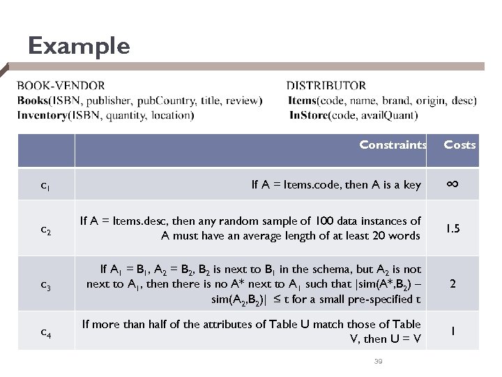Example Constraints Costs c 1 If A = Items. code, then A is a key ∞ c 2 If A = Items. desc, then any random sample of 100 data instances of A must have an average length of at least 20 words 1. 5 c 3 If A 1 = B 1, A 2 = B 2, B 2 is next to B 1 in the schema, but A 2 is not next to A 1, then there is no A* next to A 1 such that |sim(A*, B 2) – sim(A 2, B 2)| ≤ t for a small pre-specified t 2 c 4 If more than half of the attributes of Table U match those of Table V, then U = V 1 39

Domain Integrity Constraints § Each constraint is specified only once by the designer § Key requirement § given a constraint c and a match combination M, the enforce must be able to efficiently decide whether M violates c, given all the available data instances of the schemas § If the enforcer cannot detect a violation, that does not mean that the constraint indeed holds, may just mean that there is not enough data to verify § e. g. , if all current data instances of A are distinct, that does not mean A is a key 40

Searching the Space of Match Combinations § There are many ways to do this, depending on the application and the types of constraints involved § We describe here two methods § an adaptation of A* search guaranteed to find the optimal solution v but computationally more expensive v § local propagation faster v but performs only local optimizations v 41

Review: A* Search § A* searches for a goal state within a set of states, beginning from an initial state § Each path through the search space is assigned a cost § A* finds the goal state with the cheapest path from the initial state § Performs best-first search § § starts with the initial state, expand this state into a set of states selects the state with the smallest estimated cost expands the selected state into a set of states again selects the state with the smallest estimated cost, etc. 42

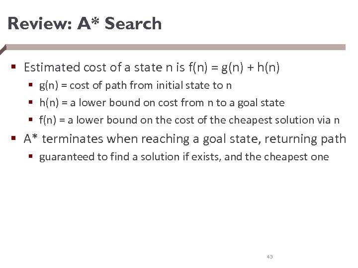Review: A* Search § Estimated cost of a state n is f(n) = g(n) + h(n) § g(n) = cost of path from initial state to n § h(n) = a lower bound on cost from n to a goal state § f(n) = a lower bound on the cost of the cheapest solution via n § A* terminates when reaching a goal state, returning path § guaranteed to find a solution if exists, and the cheapest one 43

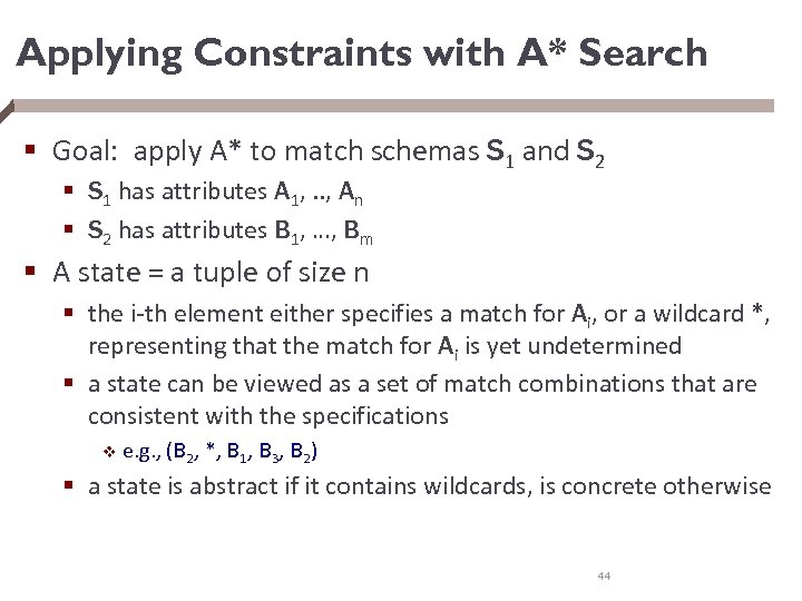Applying Constraints with A* Search § Goal: apply A* to match schemas S 1 and S 2 § S 1 has attributes A 1, . . , An § S 2 has attributes B 1, …, Bm § A state = a tuple of size n § the i-th element either specifies a match for Ai, or a wildcard *, representing that the match for Ai is yet undetermined § a state can be viewed as a set of match combinations that are consistent with the specifications v e. g. , (B 2, *, B 1, B 3, B 2) § a state is abstract if it contains wildcards, is concrete otherwise 44

Applying Constraints with A* Search § Initial state: (*, *, …, *) = all match combinations § Goal states: those that do not contain any * § Expanding states: § can only expand an abstract state § choose a * and replace it with all possible matches § a key decision is which * to expand 45

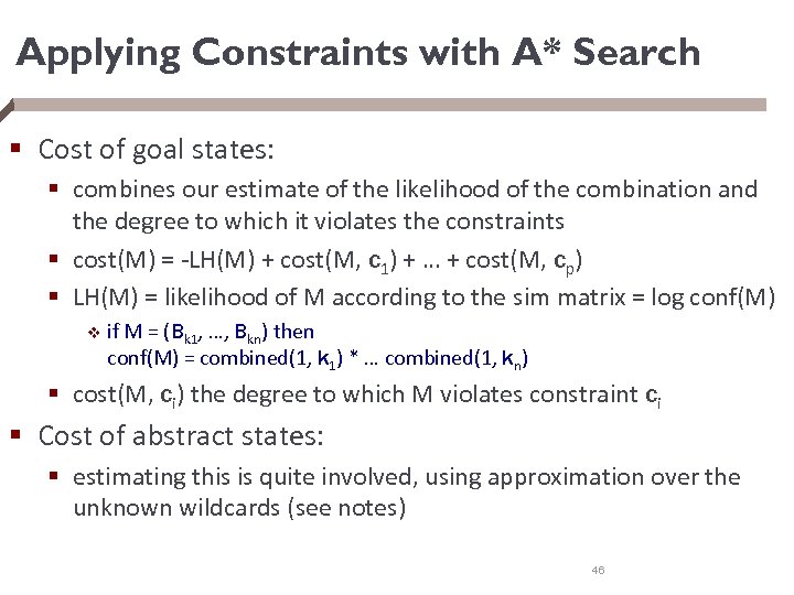Applying Constraints with A* Search § Cost of goal states: § combines our estimate of the likelihood of the combination and the degree to which it violates the constraints § cost(M) = -LH(M) + cost(M, c 1) + … + cost(M, cp) § LH(M) = likelihood of M according to the sim matrix = log conf(M) v if M = (Bk 1, …, Bkn) then conf(M) = combined(1, k 1) * … combined(1, kn) § cost(M, ci) the degree to which M violates constraint ci § Cost of abstract states: § estimating this is quite involved, using approximation over the unknown wildcards (see notes) 46

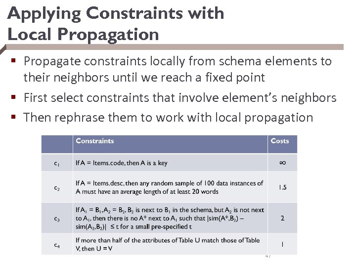Applying Constraints with Local Propagation § Propagate constraints locally from schema elements to their neighbors until we reach a fixed point § First select constraints that involve element’s neighbors § Then rephrase them to work with local propagation 47

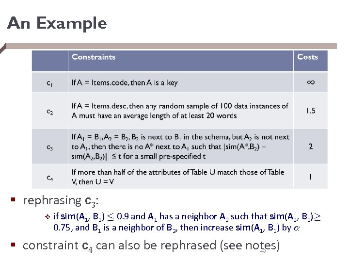An Example § rephrasing c 3: v if sim(A 1, B 1) · 0. 9 and A 1 has a neighbor A 2 such that sim(A 2, B 2)¸ 0. 75, and B 1 is a neighbor of B 2, then increase sim(A 1, B 1) by ® § constraint c 4 can also be rephrased (see notes) 48

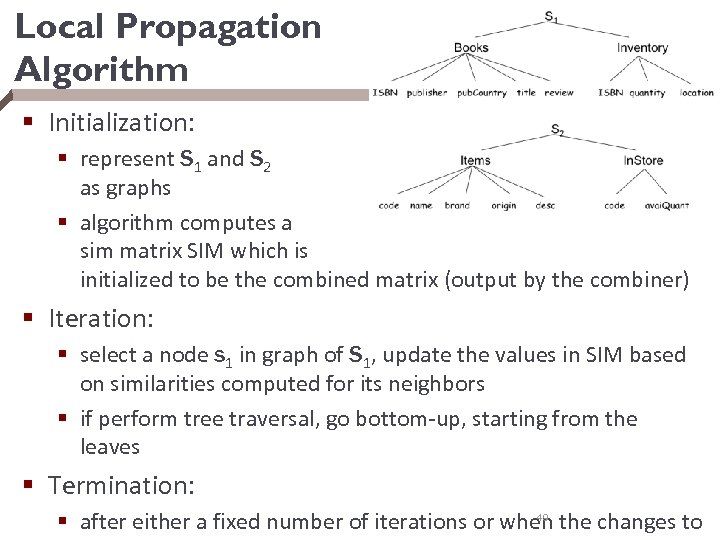Local Propagation Algorithm § Initialization: § represent S 1 and S 2 as graphs § algorithm computes a sim matrix SIM which is initialized to be the combined matrix (output by the combiner) § Iteration: § select a node s 1 in graph of S 1, update the values in SIM based on similarities computed for its neighbors § if perform tree traversal, go bottom-up, starting from the leaves § Termination: 49 § after either a fixed number of iterations or when the changes to

Reminder: Matching System Architecture 50

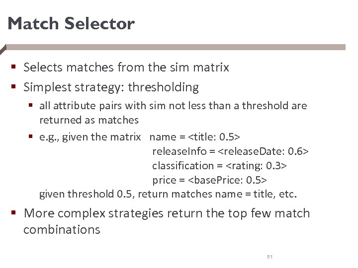Match Selector § Selects matches from the sim matrix § Simplest strategy: thresholding § all attribute pairs with sim not less than a threshold are returned as matches § e. g. , given the matrix name = release. Info = classification = price = given threshold 0. 5, return matches name = title, etc. § More complex strategies return the top few match combinations 51

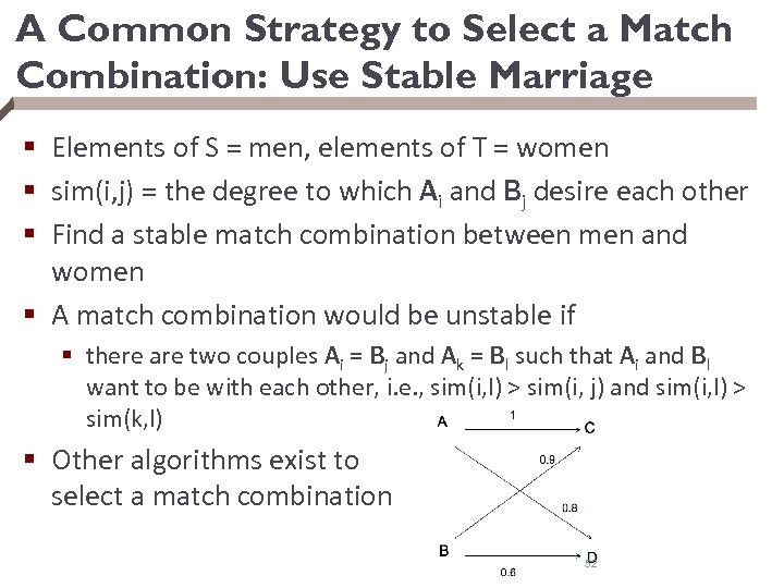A Common Strategy to Select a Match Combination: Use Stable Marriage § Elements of S = men, elements of T = women § sim(i, j) = the degree to which Ai and Bj desire each other § Find a stable match combination between men and women § A match combination would be unstable if § there are two couples Ai = Bj and Ak = Bl such that Ai and Bl want to be with each other, i. e. , sim(i, l) > sim(i, j) and sim(i, l) > sim(k, l) § Other algorithms exist to select a match combination 52

Outline § Problem definition, challenges, and overview § Schema matching § § § Matchers Combining match predictions Enforcing domain integrity constraints Match selector Reusing previous matches Many-to-many matches § Schema mapping 53

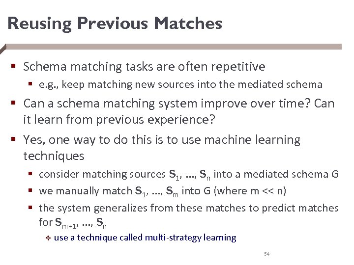Reusing Previous Matches § Schema matching tasks are often repetitive § e. g. , keep matching new sources into the mediated schema § Can a schema matching system improve over time? Can it learn from previous experience? § Yes, one way to do this is to use machine learning techniques § consider matching sources S 1, . . . , Sn into a mediated schema G § we manually match S 1, . . . , Sm into G (where m << n) § the system generalizes from these matches to predict matches for Sm+1, . . . , Sn v use a technique called multi-strategy learning 54

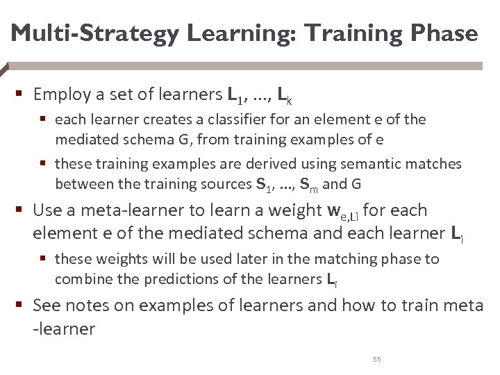Multi-Strategy Learning: Training Phase § Employ a set of learners L 1, . . . , Lk § each learner creates a classifier for an element e of the mediated schema G, from training examples of e § these training examples are derived using semantic matches between the training sources S 1, . . . , Sm and G § Use a meta-learner to learn a weight we, Li for each element e of the mediated schema and each learner Li § these weights will be used later in the matching phase to combine the predictions of the learners Li § See notes on examples of learners and how to train meta -learner 55

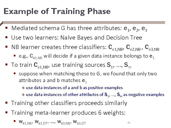Example of Training Phase § Mediated schema G has three attributes: e 1, e 2, e 3 § Use two learners: Naive Bayes and Decision Tree § NB learner creates three classifiers: Ce 1, NB, Ce 2, NB , Ce 3, NB § e. g. , Ce 1, NB will decide if a given data instance belongs to e 1 § To train Ce 1, NB, use training sources S 1, . . . , Sm § suppose when matching these to G, we found that only two attributes a and b matches e 1 use data instances of a and b as positive examples v use data instances of other attributes of S 1, . . . , Sm as negative examples v § Training other classifiers proceeds similarly § Training meta-learner produces 6 weights: § we 1, NB, we 1, DT, . . . , we 3, NB, we 3, DT 56

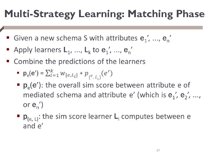Multi-Strategy Learning: Matching Phase § 57

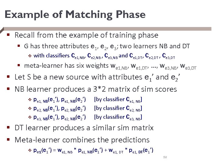Example of Matching Phase § Recall from the example of training phase § G has three attributes e 1, e 2, e 3; two learners NB and DT v with classifiers Ce 1, NB, Ce 2, NB , Ce 3, NB and Ce 1, DT, Ce 2, DT , Ce 3, DT § meta-learner has six weights we 1, NB, we 1, DT, . . . , we 3, NB, we 3, DT § Let S be a new source with attributes e 1’ and e 2’ § NB learner produces a 3*2 matrix of sim scores pe 1, NB(e 1’), pe 1, NB(e 2’) [by classifier Ce 1, NB] v pe 2, NB(e 1’), pe 2, NB(e 2’) [by classifier Ce 2, NB] v pe 3, NB(e 1’), pe 2, NB(e 2’) [by classifier Ce 3, NB] v § DT learner produces a similar sim matrix § Meta-learner combines the predictions v pe 1(e 1’) = we 1, NB * pe 1, NB(e 1’) + we 1, DT * pe 1, DT(e 1’) 58

Discussion § Mapping to the generic schema matching architecture § learners = matchers § meta-learner = combiner § Here the matchers and combiner use machine learning techniques enable them to learn from previous matching experiences (of sources S 1, . . . , Sm) § Note that even when we match just two souces S and T, we can still use machine learning techniques in the matchers and combiners § e. g. , if the data instances of source S are available, they can be used as training data to build classifiers over S 59

Outline § Problem definition, challenges, and overview § Schema matching § § § Matchers Combining match predictions Enforcing domain integrity constraints Match selector Reusing previous matches Many-to-many matches § Schema mapping 60

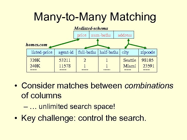Many-to-Many Matching Mediated-schema price num-baths address homes. com listed-price 320 K 240 K agent-id 53211 11578 full-baths half-baths city 2 1 1 1 Seattle Miami zipcode 98105 23591 • Consider matches between combinations of columns – … unlimited search space! • Key challenge: control the search.

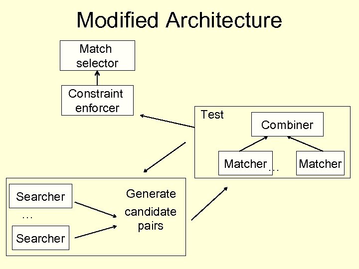
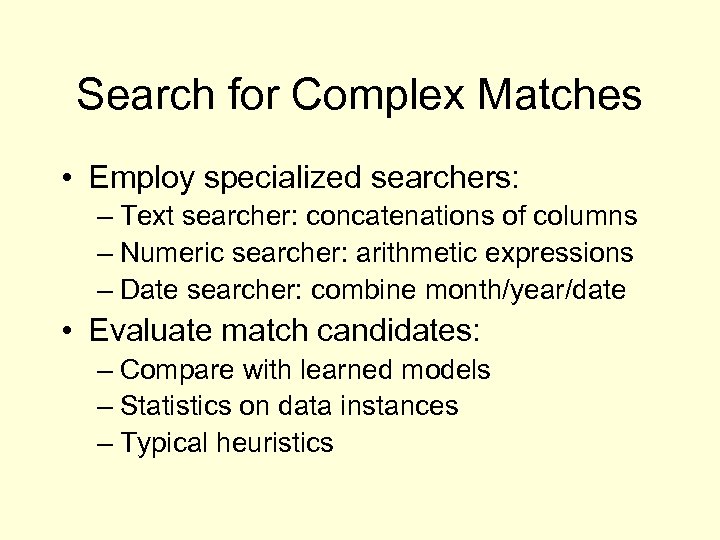Search for Complex Matches • Employ specialized searchers: – Text searcher: concatenations of columns – Numeric searcher: arithmetic expressions – Date searcher: combine month/year/date • Evaluate match candidates: – Compare with learned models – Statistics on data instances – Typical heuristics

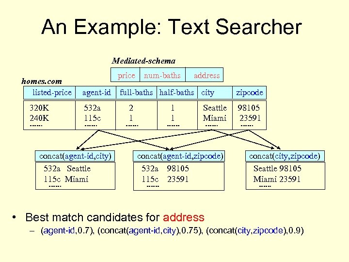An Example: Text Searcher Mediated-schema homes. com listed-price 320 K 240 K price agent-id 532 a 115 c concat(agent-id, city) 532 a Seattle 115 c Miami num-baths address full-baths half-baths city 2 1 1 1 Seattle Miami concat(agent-id, zipcode) 532 a 98105 115 c 23591 zipcode 98105 23591 concat(city, zipcode) Seattle 98105 Miami 23591 • Best match candidates for address – (agent-id, 0. 7), (concat(agent-id, city), 0. 75), (concat(city, zipcode), 0. 9)

Controlling the Search • Limit the search with beam search: – Consider only top k candidates at every level of the search • Termination based on diminishing returns: – Estimate of quality does not change much between iterations • Details of a system that did this: – i. Map [Doan et al. , SIGMOD, 2004]

Modified Architecture Match selector Constraint enforcer Test Combiner Matcher … Searcher Generate candidate pairs Matcher

Outline § Problem definition, challenges, and overview § Schema matching § § § Matchers Combining match predictions Enforcing domain integrity constraints Match selector Reusing previous matches Many-to-many matches § Schema mapping 66

From Matching to Mapping • Input: – Schema matches – Constraints (if available) • Output: – Schema mappings – (for now, let’s do SQL) • Let’s look at the choices we need to make – A solution will emerge… – Based on the IBM Clio Project

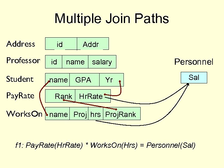Multiple Join Paths Address id Addr Professor id Student name GPA Pay. Rate name salary Yr Personnel Sal Rank Hr. Rate Works. On name Proj hrs Proj. Rank f 1: Pay. Rate(Hr. Rate) * Works. On(Hrs) = Personnel(Sal)

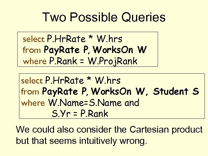Two Possible Queries select P. Hr. Rate * W. hrs from Pay. Rate P, Works. On W where P. Rank = W. Proj. Rank select P. Hr. Rate * W. hrs from Pay. Rate P, Works. On W, Student S where W. Name=S. Name and S. Yr = P. Rank We could also consider the Cartesian product but that seems intuitively wrong.

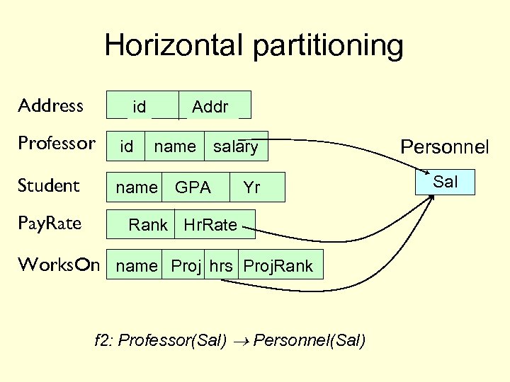Horizontal partitioning Address id Addr Professor id Student name GPA Pay. Rate name salary Yr Rank Hr. Rate Works. On name Proj hrs Proj. Rank f 2: Professor(Sal) Personnel(Sal) Personnel Sal

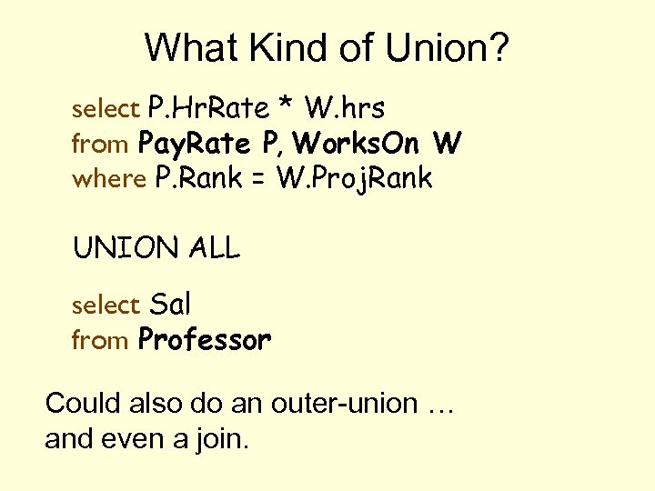What Kind of Union? select P. Hr. Rate * W. hrs from Pay. Rate P, Works. On W where P. Rank = W. Proj. Rank UNION ALL select Sal from Professor Could also do an outer-union … and even a join.

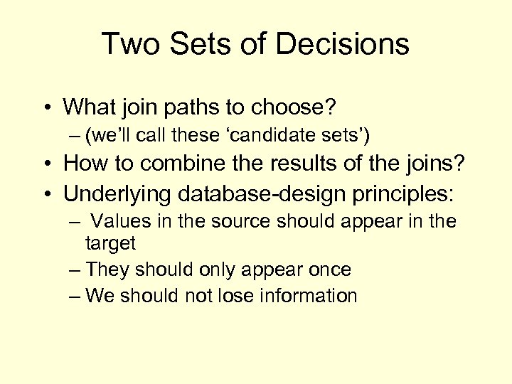Two Sets of Decisions • What join paths to choose? – (we’ll call these ‘candidate sets’) • How to combine the results of the joins? • Underlying database-design principles: – Values in the source should appear in the target – They should only appear once – We should not lose information

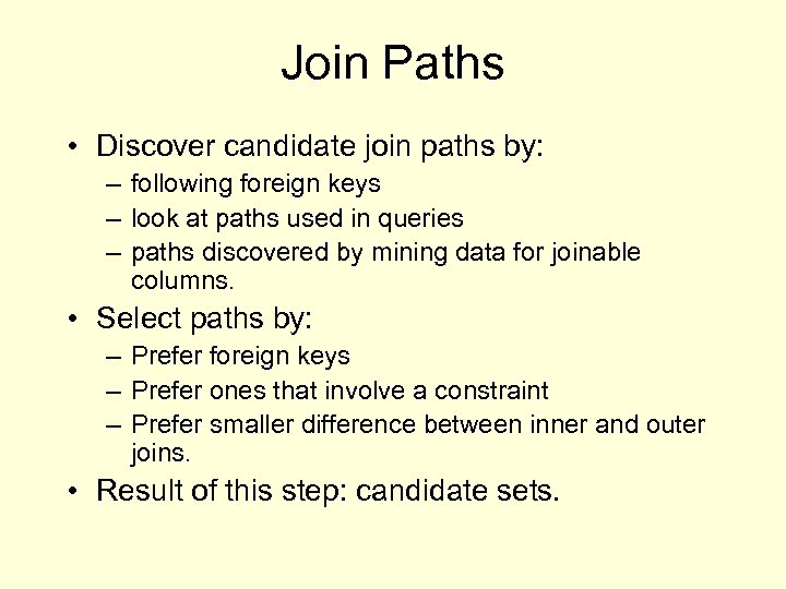Join Paths • Discover candidate join paths by: – following foreign keys – look at paths used in queries – paths discovered by mining data for joinable columns. • Select paths by: – Prefer foreign keys – Prefer ones that involve a constraint – Prefer smaller difference between inner and outer joins. • Result of this step: candidate sets.

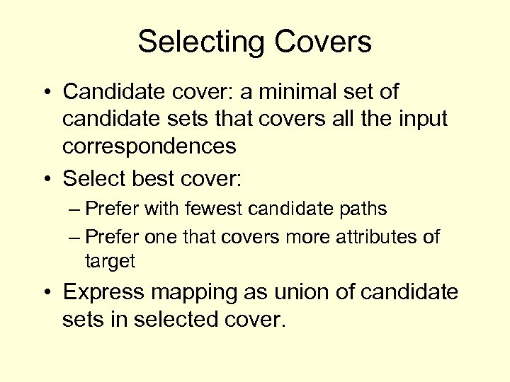Selecting Covers • Candidate cover: a minimal set of candidate sets that covers all the input correspondences • Select best cover: – Prefer with fewest candidate paths – Prefer one that covers more attributes of target • Express mapping as union of candidate sets in selected cover.

Summary • Schema matching: – Use multiple matchers and combine results – Learn from the past – Incorporate constraints and user feedback • From matching to mapping: – Search through possible queries – Principles from database design guide search – User interaction is key