Chapter 5 Risk and Return Past and Prologue

Chapter 5 Risk and Return: Past and Prologue Mc. Graw-Hill/Irwin Copyright © 2010 by The Mc. Graw-Hill Companies, Inc. All rights reserved.

5. 1 Rates of Return 5 -2

Measuring Ex-Post (Past) Returns One period investment: regardless of the length of the period. Holding period return (HPR): HPR = [PS - PB + CF] / PB where PS = Sale price (or P 1) PB = Buy price ($ you put up) (or P 0) CF = Cash flow during holding period • Q: Why use % returns at all? • Q: What are we assuming about the cash flows in the HPR calculation? 5 -3

Annualizing HPRs Q: Why would you want to annualize returns? 1. Annualizing HPRs for holding periods of greater than one year: – Without compounding (Simple or APR): HPRann = HPR/n – – With compounding: EAR HPRann = [(1+HPR)1/n]-1 where n = number of years held 5 -4

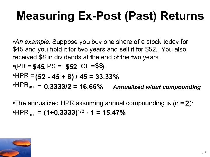Measuring Ex-Post (Past) Returns • An example: Suppose you buy one share of a stock today for $45 and you hold it for two years and sell it for $52. You also received $8 in dividends at the end of the two years. • (PB = $45, PS = $52 CF = $8): , • HPR = (52 - 45 + 8) / 45 = 33. 33% • HPRann = 0. 3333/2 = 16. 66% Annualized w/out compounding • The annualized HPR assuming annual compounding is (n = 2 ): • HPRann = (1+0. 3333)1/2 - 1 = 15. 47% 5 -5

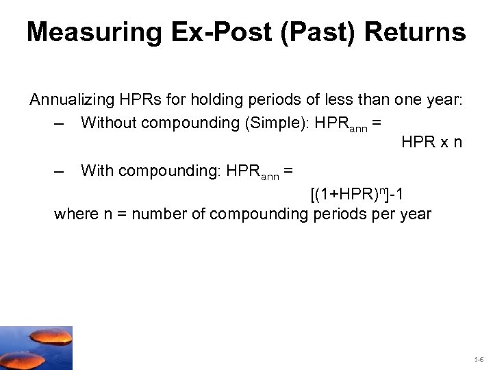Measuring Ex-Post (Past) Returns Annualizing HPRs for holding periods of less than one year: – Without compounding (Simple): HPRann = HPR x n – With compounding: HPRann = [(1+HPR)n]-1 where n = number of compounding periods per year 5 -6

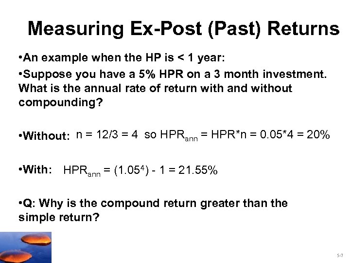Measuring Ex-Post (Past) Returns • An example when the HP is < 1 year: • Suppose you have a 5% HPR on a 3 month investment. What is the annual rate of return with and without compounding? • Without: n = 12/3 = 4 so HPRann = HPR*n = 0. 05*4 = 20% • With: HPRann = (1. 054) - 1 = 21. 55% • Q: Why is the compound return greater than the simple return? 5 -7

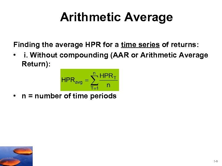Arithmetic Average Finding the average HPR for a time series of returns: • i. Without compounding (AAR or Arithmetic Average Return): • n = number of time periods 5 -8

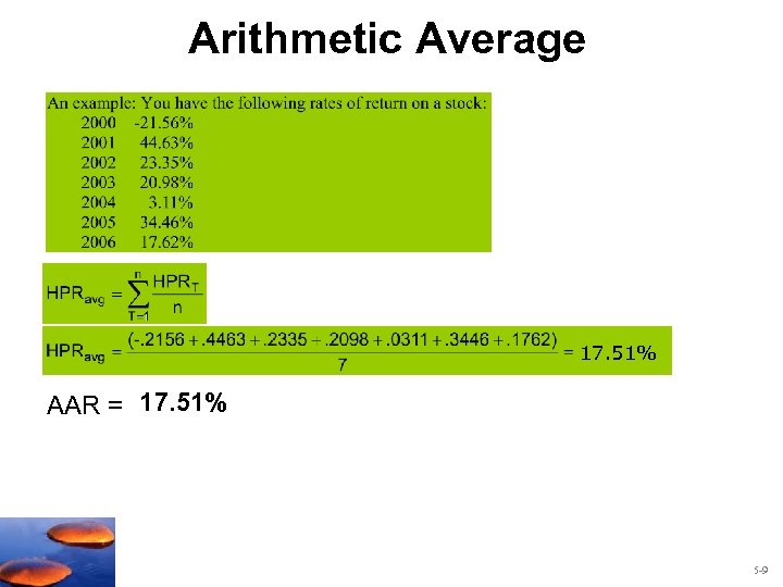Arithmetic Average 17. 51% AAR = 17. 51% 5 -9

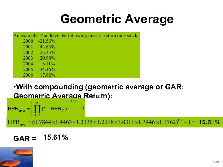Geometric Average • With compounding (geometric average or GAR: Geometric Average Return): 15. 61% GAR = 15. 61% 5 -10

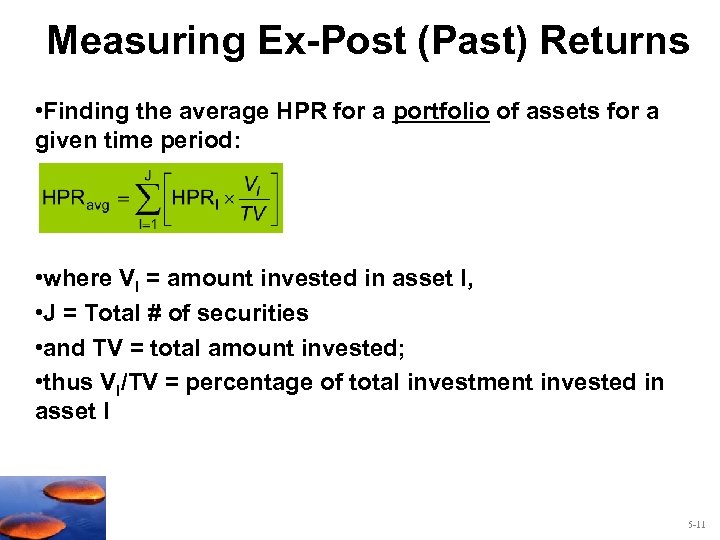Measuring Ex-Post (Past) Returns • Finding the average HPR for a portfolio of assets for a given time period: • where VI = amount invested in asset I, • J = Total # of securities • and TV = total amount invested; • thus VI/TV = percentage of total investment invested in asset I 5 -11

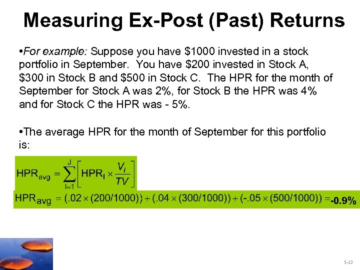Measuring Ex-Post (Past) Returns • For example: Suppose you have $1000 invested in a stock portfolio in September. You have $200 invested in Stock A, $300 in Stock B and $500 in Stock C. The HPR for the month of September for Stock A was 2%, for Stock B the HPR was 4% and for Stock C the HPR was - 5%. • The average HPR for the month of September for this portfolio is: -0. 9% 5 -12

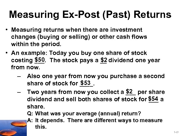Measuring Ex-Post (Past) Returns • Measuring returns when there are investment changes (buying or selling) or other cash flows within the period. • An example: Today you buy one share of stock $50 $2 costing ___. The stock pays a __ dividend one year from now. – Also one year from now you purchase a second $53 share of stock for ____. $2 – Two years from now you collect a ___ per share dividend and sell both shares of stock for $54 a ___ share. Q: What was your average (annual) return? A: It depends. There are different ways to measure this. 5 -13

Dollar-Weighted Return i. Dollar-weighted return procedure (DWR): Find the internal rate of return for the cash flows (i. e. find the discount rate that makes the NPV of the net cash flows equal zero. ) 5 -14

Tips on Calculating Dollar Weighted Returns n This measure of return considers both changes in investment and security performance n Initial Investment is an _______ outflow n Ending value is considered as an ______ inflow n Additional investment is an _______ outflow n Security sales are an ______ inflow 5 -15

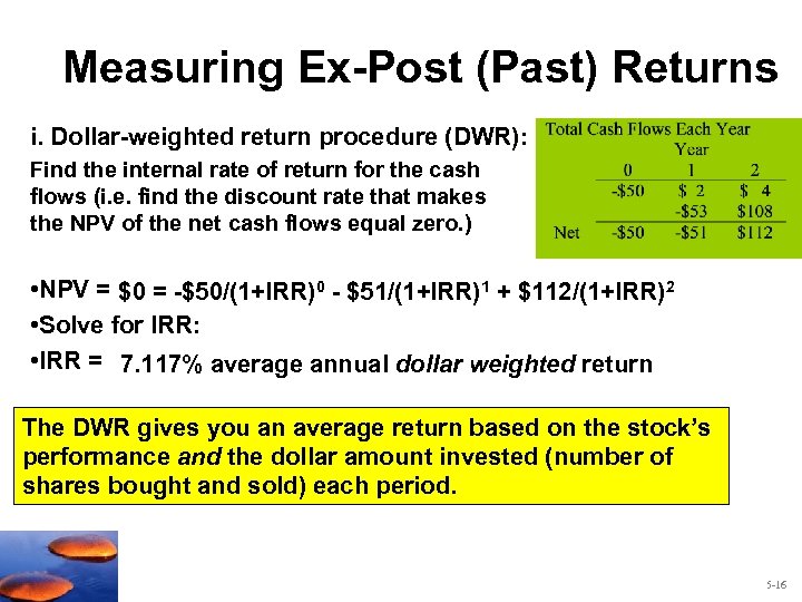Measuring Ex-Post (Past) Returns i. Dollar-weighted return procedure (DWR): Find the internal rate of return for the cash flows (i. e. find the discount rate that makes the NPV of the net cash flows equal zero. ) • NPV = $0 = -$50/(1+IRR)0 - $51/(1+IRR)1 + $112/(1+IRR)2 • Solve for IRR: • IRR = 7. 117% average annual dollar weighted return The DWR gives you an average return based on the stock’s performance and the dollar amount invested (number of shares bought and sold) each period. 5 -16

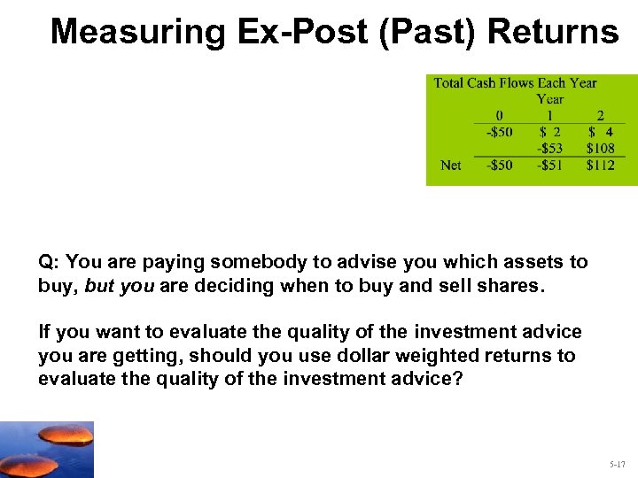Measuring Ex-Post (Past) Returns Q: You are paying somebody to advise you which assets to buy, but you are deciding when to buy and sell shares. If you want to evaluate the quality of the investment advice you are getting, should you use dollar weighted returns to evaluate the quality of the investment advice? 5 -17

Time-Weighted Returns ii. Time-weighted returns (TWR): TWRs assume you buy one share of ___ the stock at the beginning of each one interim period and sell ___ share at the end of each interim period. TWRs are thus ______ of the amount invested in a given period. independent To calculate TWRs: n Calculate the return for each time period, typically a year. n Then calculate either an arithmetic (AAR) or a geometric average (GAR) of the returns. 5 -18

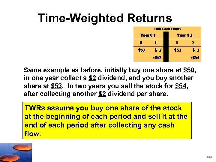Time-Weighted Returns Same example as before, initially buy one share at $50, in one year collect a $2 dividend, and you buy another share at $53. In two years you sell the stock for $54, after collecting another $2 dividend per share. TWRs assume you buy one share of the stock at the beginning of each period and sell it at the end of each period after collecting any cash flow. 5 -19

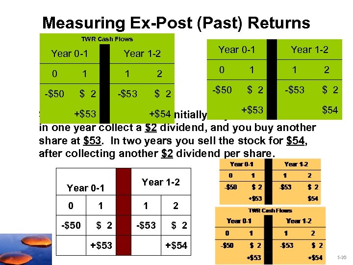Measuring Ex-Post (Past) Returns TWR Cash Flows Year 0 -1 Year 1 -2 0 1 1 -$50 $ 2 2 -$53 -$50 $ 2 1 $ 2 -$53 2 $ 2 +$53 +$54 Same example as before, initially buy one share at $50, $54 in one year collect a $2 dividend, and you buy another share at $53. In two years you sell the stock for $54, after collecting another $2 dividend per share. Year 0 -1 0 -$50 1 $ 2 +$53 Year 1 -2 1 -$53 2 $ 2 +$54 5 -20

Measuring Ex-Post (Past) Returns HPR for year 1: [$53 + $2 - $50] / $50 = 10% HPR for year 2: [$54 - $53 +$2] / $53 = 5. 66% a) Calculating the arithmetic average TW return: Arithmetic Average Return (AAR): Calculate the arithmetic average AAR = [0. 10 + 0. 0566] / 2 = 7. 83% 5 -21

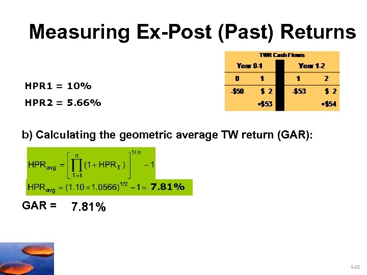Measuring Ex-Post (Past) Returns HPR 1 = 10% HPR 2 = 5. 66% b) Calculating the geometric average TW return (GAR): 7. 81% GAR = 7. 81% 5 -22

Measuring Ex-Post (Past) Returns Q: When should you use the GAR and when should you use the AAR? A 1: When you are evaluating PAST RESULTS (ex-post): n Use the AAR (average without compounding) if you ARE NOT reinvesting any cash flows received before the end of the period. n Use the GAR (average with compounding) if you ARE reinvesting any cash flows received before the end of the period. A 2: When you are trying to estimate an expected return (exante return): n Use the AAR 5 -23

5. 2 Risk and Risk Premiums 5 -24

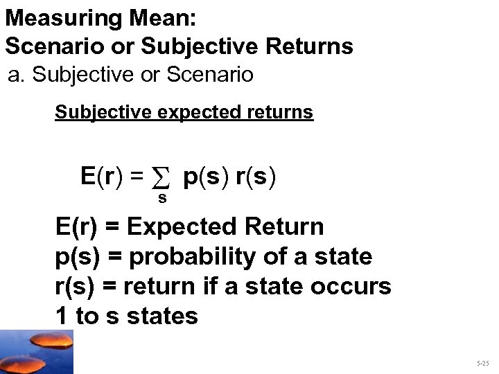Measuring Mean: Scenario or Subjective Returns a. Subjective or Scenario Subjective expected returns E(r) = p(s) r(s) s E(r) = Expected Return p(s) = probability of a state r(s) = return if a state occurs 1 to s states 5 -25

Measuring Variance or Dispersion of Returns a. Subjective or Scenario Variance = [ 2]1/2 E(r) = Expected Return p(s) = probability of a state rs = return in state “s” 5 -26

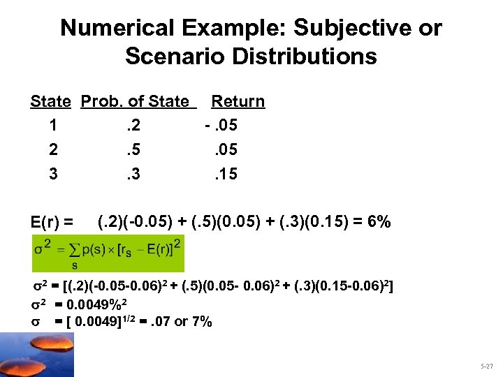Numerical Example: Subjective or Scenario Distributions State Prob. of State Return 1. 2 -. 05 2. 5. 05 3. 3. 15 E(r) = (. 2)(-0. 05) + (. 5)(0. 05) + (. 3)(0. 15) = 6% 2 = [(. 2)(-0. 05 -0. 06)2 + (. 5)(0. 05 - 0. 06)2 + (. 3)(0. 15 -0. 06)2] 2 = 0. 0049%2 = [ 0. 0049]1/2 =. 07 or 7% 5 -27

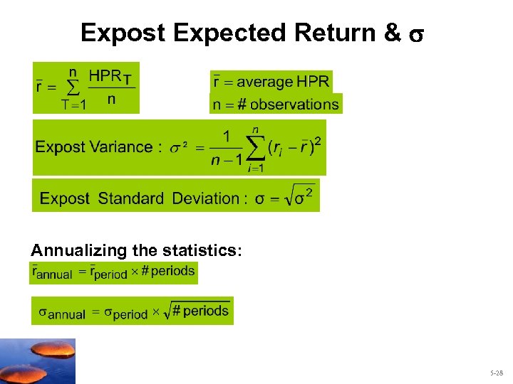Expost Expected Return & Annualizing the statistics: 5 -28

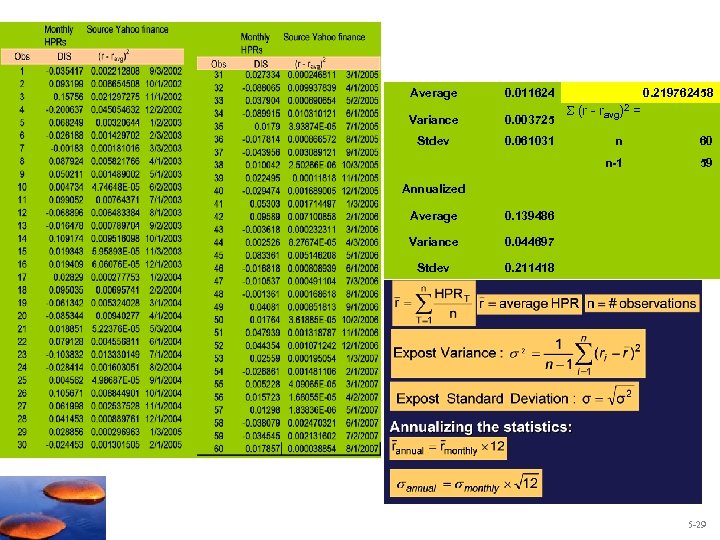Average 0. 011624 Variance 0. 003725 Stdev 0. 061031 0. 219762458 (r - ravg)2 = n 60 n-1 59 Annualized Average 0. 139486 Variance 0. 044697 Stdev 0. 211418 5 -29

Using Ex-Post Returns to estimate Expected HPR Estimating Expected HPR (E[r]) from ex-post data. Use the arithmetic average of past returns as a forecast of expected future returns as we did and, Perhaps apply some (usually ad-hoc) adjustment to past returns • Which historical time period? Problems? • Have to adjust for current economic situation • Unstable averages • Stable risk 5 -30

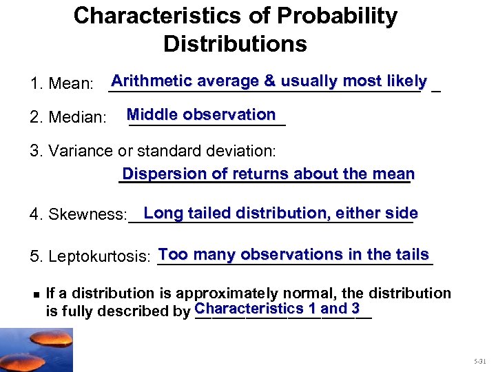Characteristics of Probability Distributions Arithmetic average & usually most likely 1. Mean: _________________ _ 2. Median: Middle observation _________ 3. Variance or standard deviation: Dispersion of returns about the mean Long tailed distribution, either side 4. Skewness: ________________ Too many observations in the tails 5. Leptokurtosis: _______________ n If a distribution is approximately normal, the distribution is fully described by Characteristics 1 and 3 ___________ 5 -31

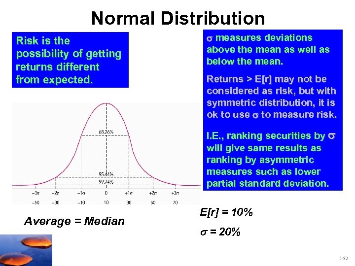Normal Distribution Risk is the possibility of getting returns different from expected. measures deviations above the mean as well as below the mean. Returns > E[r] may not be considered as risk, but with symmetric distribution, it is ok to use to measure risk. I. E. , ranking securities by will give same results as ranking by asymmetric measures such as lower partial standard deviation. Average = Median E[r] = 10% = 20% 5 -32

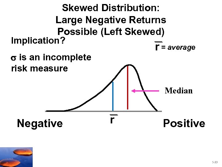Skewed Distribution: Large Negative Returns Possible (Left Skewed) Implication? r = average is an incomplete risk measure Median Negative r Positive 5 -33

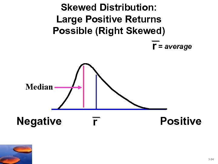Skewed Distribution: Large Positive Returns Possible (Right Skewed) r = average Median Negative r Positive 5 -34

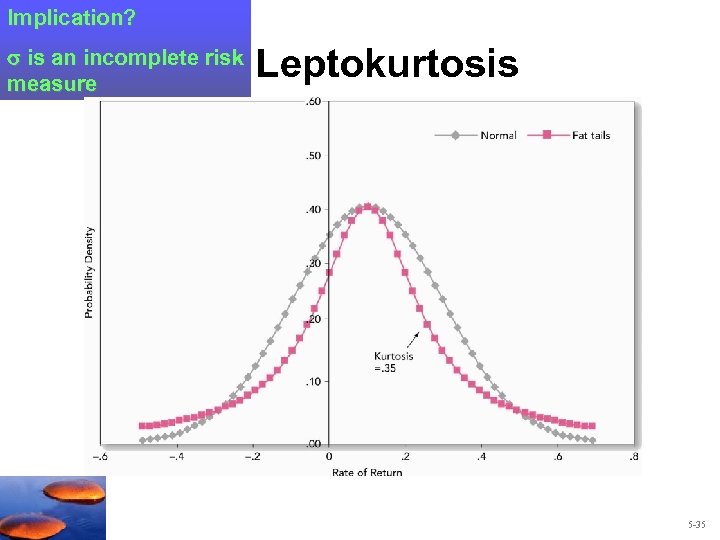Implication? is an incomplete risk measure Leptokurtosis 5 -35

Value at Risk (Va. R) Value at Risk attempts to answer the following question: • How many dollars can I expect to lose on my portfolio in a given time period at a given level of probability? • The typical probability used is 5%. • We need to know what HPR corresponds to a 5% probability. • If returns are normally distributed then we can use a standard normal table or Excel to determine how many standard deviations below the mean represents a 5% probability: – From Excel: =Norminv (0. 05, 0, 1) = -1. 64485 standard deviations 5 -36

Value at Risk (Va. R) From the standard deviation we can find the corresponding level of the portfolio return: Va. R = E[r] + -1. 64485 For Example: A $500, 000 stock portfolio has an annual expected return of 12% and a standard deviation of 35%. What is the portfolio Va. R at a 5% probability level? Va. R = 0. 12 + (-1. 64485 * 0. 35) Va. R = -45. 57% (rounded slightly) Va. R$ = $500, 000 x -. 4557 = -$227, 850 What does this number mean? 5 -37

Value at Risk (Va. R) Va. R versus standard deviation: • For normally distributed returns Va. R is equivalent to standard deviation (although Va. R is typically reported in dollars rather than in % returns) • Va. R adds value as a risk measure when return distributions are not normally distributed. – Actual 5% probability level will differ from 1. 68445 standard deviations from the mean due to kurtosis and skewness. 5 -38

Risk Premium & Risk Aversion • The risk free rate is the rate of return that can be earned with certainty. • The risk premium is the difference between the expected return of a risky asset and the risk-free rate. E[rasset] – rf Excess Return or Risk Premiumasset = Risk aversion is an investor’s reluctance to accept risk. How is the aversion to accept risk overcome? By offering investors a higher risk premium. 5 -39

5. 3 The Historical Record 5 -40

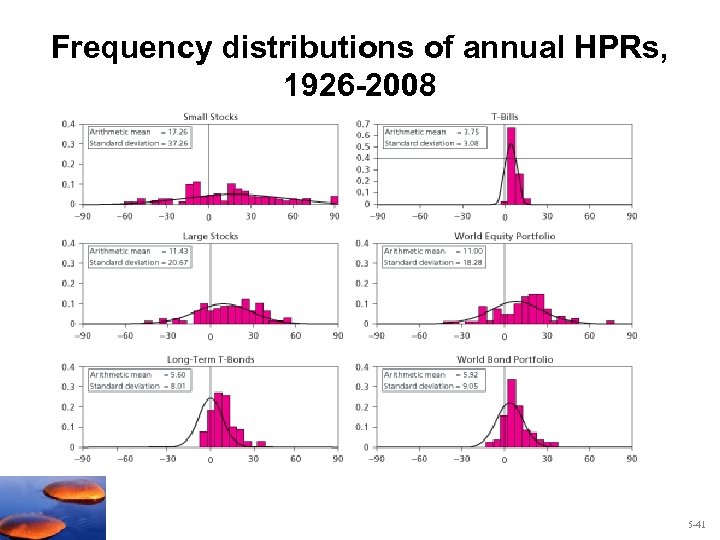Frequency distributions of annual HPRs, 1926 -2008 5 -41

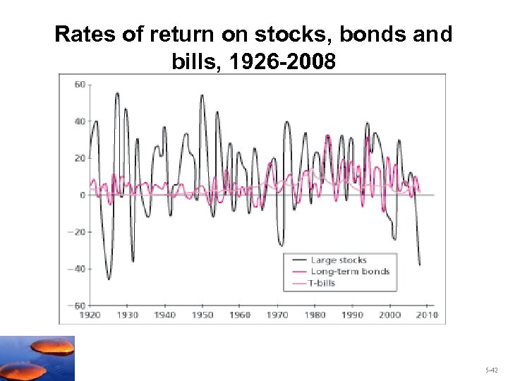Rates of return on stocks, bonds and bills, 1926 -2008 5 -42

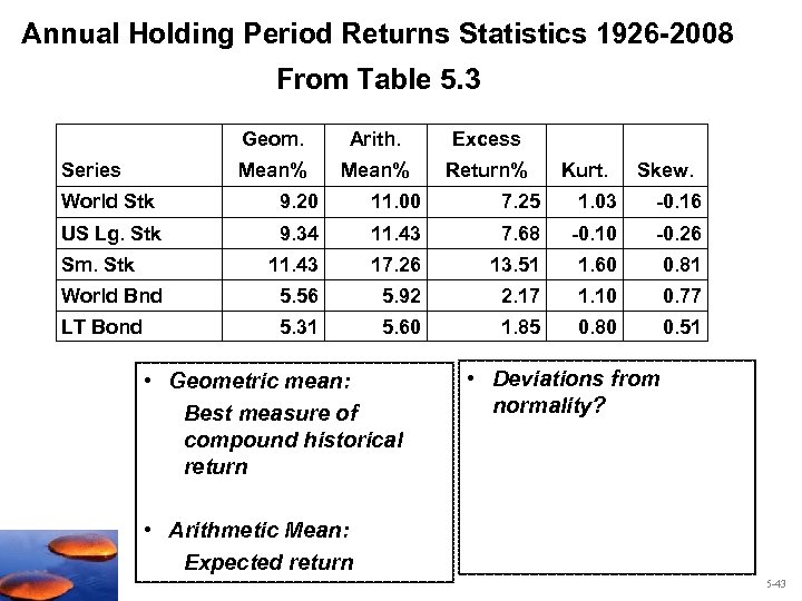Annual Holding Period Returns Statistics 1926 -2008 From Table 5. 3 Geom. Excess Mean% Series Arith. Mean% Return% Kurt. Skew. World Stk 9. 20 11. 00 7. 25 1. 03 -0. 16 US Lg. Stk 9. 34 11. 43 7. 68 -0. 10 -0. 26 11. 43 17. 26 13. 51 1. 60 0. 81 World Bnd 5. 56 5. 92 2. 17 1. 10 0. 77 LT Bond 5. 31 5. 60 1. 85 0. 80 0. 51 Sm. Stk • Geometric mean: Best measure of compound historical return • Deviations from normality? • Arithmetic Mean: Expected return 5 -43

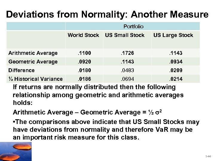Deviations from Normality: Another Measure Portfolio World Stock US Small Stock US Large Stock Arithmetic Average . 1100 . 1726 . 1143 Geometric Average . 0920 . 1143 . 0934 Difference . 0180 . 0483 . 0209 ½ Historical Variance . 0186 . 0694 . 0214 If returns are normally distributed then the following relationship among geometric and arithmetic averages holds: Arithmetic Average – Geometric Average = ½ 2 • The comparisons above indicate that US Small Stocks may have deviations from normality and therefore Va. R may be an important risk measure for this class. 5 -44

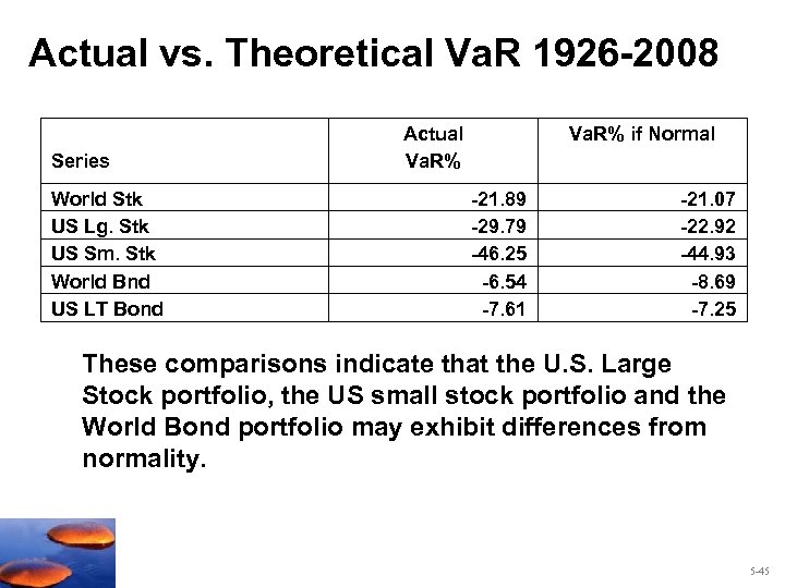Actual vs. Theoretical Va. R 1926 -2008 Series World Stk US Lg. Stk US Sm. Stk World Bnd US LT Bond Actual Va. R% if Normal -21. 89 -29. 79 -46. 25 -6. 54 -7. 61 -21. 07 -22. 92 -44. 93 -8. 69 -7. 25 These comparisons indicate that the U. S. Large Stock portfolio, the US small stock portfolio and the World Bond portfolio may exhibit differences from normality. 5 -45

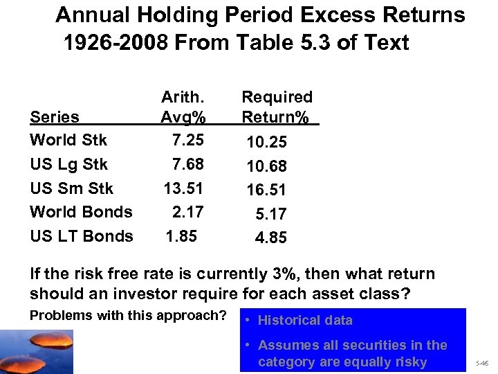Annual Holding Period Excess Returns 1926 -2008 From Table 5. 3 of Text Series World Stk US Lg Stk US Sm Stk World Bonds US LT Bonds Arith. Avg% 7. 25 7. 68 13. 51 2. 17 1. 85 Required Return% 10. 25 10. 68 16. 51 5. 17 4. 85 If the risk free rate is currently 3%, then what return should an investor require for each asset class? Problems with this approach? • Historical data • Assumes all securities in the category are equally risky 5 -46

5. 4 Inflation and Real Rates of Return 5 -47

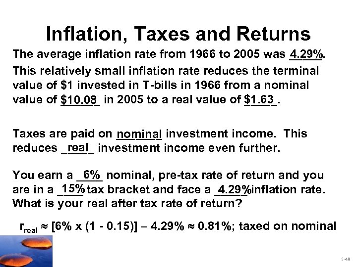Inflation, Taxes and Returns The average inflation rate from 1966 to 2005 was _____. 4. 29% This relatively small inflation rate reduces the terminal value of $1 invested in T-bills in 1966 from a nominal value of ______ in 2005 to a real value of $1. 63 _____. $10. 08 Taxes are paid on _______ investment income. This nominal reduces _____ investment income even further. 6% You earn a ____ nominal, pre-tax rate of return and you 15% are in a ____ tax bracket and face a _____ inflation rate. 4. 29% What is your real after tax rate of return? rreal [6% x (1 - 0. 15)] – 4. 29% 0. 81%; taxed on nominal 5 -48

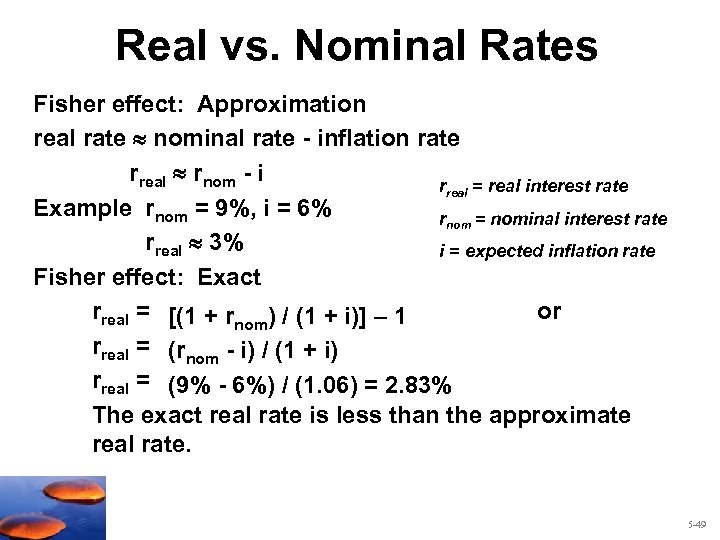Real vs. Nominal Rates Fisher effect: Approximation real rate nominal rate - inflation rate rreal rnom - i rreal = real interest rate Example rnom = 9%, i = 6% rnom = nominal interest rate rreal 3% i = expected inflation rate Fisher effect: Exact rreal = [(1 + rnom) / (1 + i)] – 1 or rreal = (rnom - i) / (1 + i) rreal = (9% - 6%) / (1. 06) = 2. 83% The exact real rate is less than the approximate real rate. 5 -49

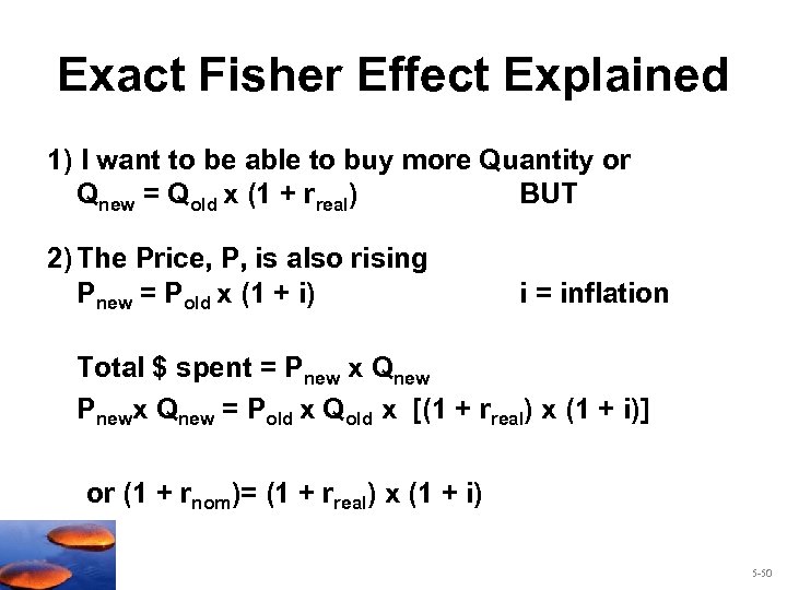Exact Fisher Effect Explained 1) I want to be able to buy more Quantity or Qnew = Qold x (1 + rreal) BUT 2) The Price, P, is also rising Pnew = Pold x (1 + i) i = inflation Total $ spent = Pnew x Qnew Pnewx Qnew = Pold x Qold x [(1 + rreal) x (1 + i)] or (1 + rnom)= (1 + rreal) x (1 + i) 5 -50

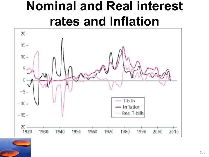Nominal and Real interest rates and Inflation 5 -51

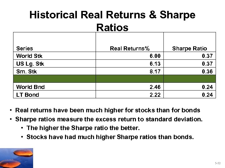Historical Returns & Sharpe Ratios Series World Stk US Lg. Stk Sm. Stk World Bnd LT Bond Real Returns% 6. 00 6. 13 8. 17 Sharpe Ratio 0. 37 0. 36 2. 46 2. 22 0. 24 • Real returns have been much higher for stocks than for bonds • Sharpe ratios measure the excess return to standard deviation. • The higher the Sharpe ratio the better. • Stocks have had much higher Sharpe ratios than bonds. 5 -52

5. 5 Asset Allocation Across Risky and Risk Free Portfolios 5 -53

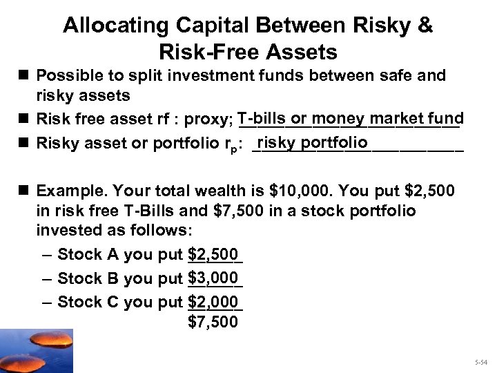Allocating Capital Between Risky & Risk-Free Assets n Possible to split investment funds between safe and risky assets n Risk free asset rf : proxy; T-bills or money market fund ____________ risky portfolio n Risky asset or portfolio rp: ____________ n Example. Your total wealth is $10, 000. You put $2, 500 in risk free T-Bills and $7, 500 in a stock portfolio invested as follows: – Stock A you put $2, 500 ______ – Stock B you put $3, 000 ______ – Stock C you put $2, 000 ______ $7, 500 5 -54

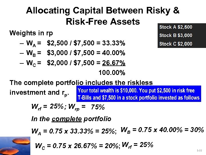Allocating Capital Between Risky & Risk-Free Assets Weights in rp – WA = $2, 500 / $7, 500 = 33. 33% – WB = $3, 000 / $7, 500 = 40. 00% – WC = $2, 000 / $7, 500 = 26. 67% 100. 00% The complete portfolio includes the riskless investment and rp. Wrf = 25% ; Wrp = 75% In the complete portfolio WA = 0. 75 x 33. 33% = 25%; WB = 0. 75 x 40. 00% = 30% WC = 0. 75 x 26. 67% = 20%; Wrf = 25% 5 -55

Allocating Capital Between Risky & Risk-Free Assets • Issues in setting weights risk & return tradeoff – Examine __________ – Demonstrate how different degrees of risk allocations aversion will affect _____ between risky and risk free assets 5 -56

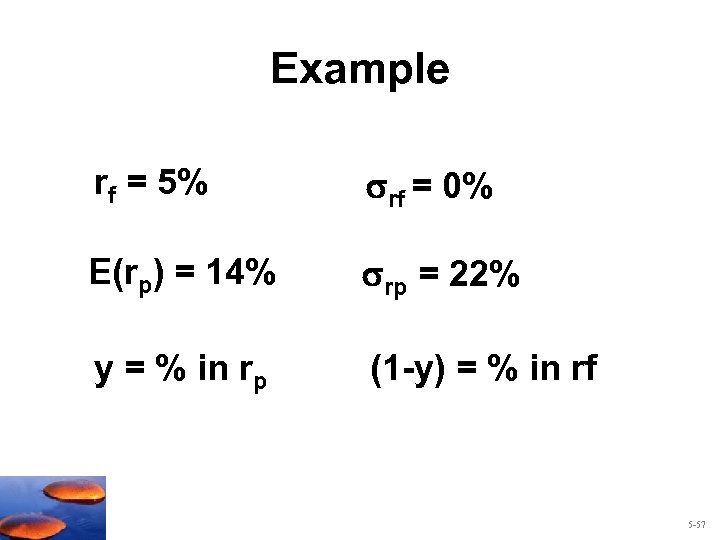Example rf = 5% rf = 0% E(rp) = 14% rp = 22% y = % in rp (1 -y) = % in rf 5 -57

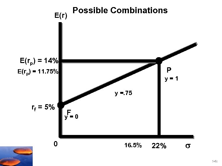
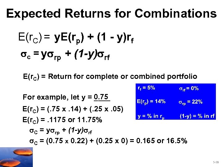Expected Returns for Combinations E(r. C) = y. E(rp) + (1 - y)rf c = y rp + (1 -y) rf E(r. C) = Return for complete or combined portfolio For example, let y = 0. 75 ____ E(r. C) = (. 75 x. 14) + (. 25 x. 05) E(r. C) =. 1175 or 11. 75% C = y rp + (1 -y) rf C = (0. 75 x 0. 22) + (0. 25 x 0) = 0. 165 or 16. 5% 5 -58

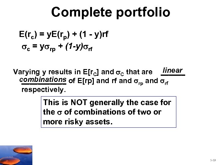Complete portfolio E(rc) = y. E(rp) + (1 - y)rf c = y rp + (1 -y) rf linear Varying y results in E[r. C] and C that are ______ combinations of E[rp] and rf and rp and rf ______ respectively. This is NOT generally the case for the of combinations of two or more risky assets. 5 -59

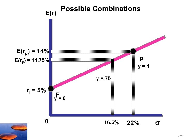E(r) Possible Combinations E(rp) = 14% P E(rp) = 11. 75% y=1 y =. 75 rf = 5% F y=0 0 16. 5% 22% 5 -60

E(r) Possible Combinations E(rp) = 14% P E(rp) = 11. 75% y=1 y =. 75 rf = 5% F y=0 0 16. 5% 22% 5 -61

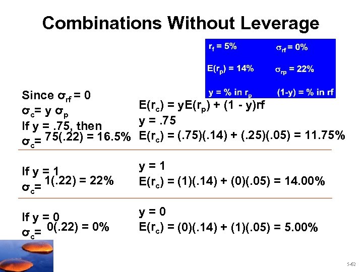Combinations Without Leverage Since σrf = 0 E(rc) = y. E(rp) + (1 - y)rf σc= y σp y =. 75 If y =. 75, then σc= 75(. 22) = 16. 5% E(rc) = (. 75)(. 14) + (. 25)(. 05) = 11. 75% If y = 1 1(. 22) = 22% σc= y=1 E(rc) = (1)(. 14) + (0)(. 05) = 14. 00% If y = 0 σc= 0(. 22) = 0% y=0 E(rc) = (0)(. 14) + (1)(. 05) = 5. 00% 5 -62

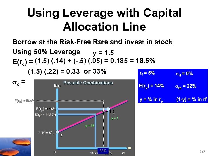Using Leverage with Capital Allocation Line Borrow at the Risk-Free Rate and invest in stock Using 50% Leverage y = 1. 5 E(rc) = (1. 5) (. 14) + (-. 5) (. 05) = 0. 185 = 18. 5% (1. 5) (. 22) = 0. 33 or 33% c = E(r. C) =18. 5% y = 1. 5 y=0 33% 5 -63

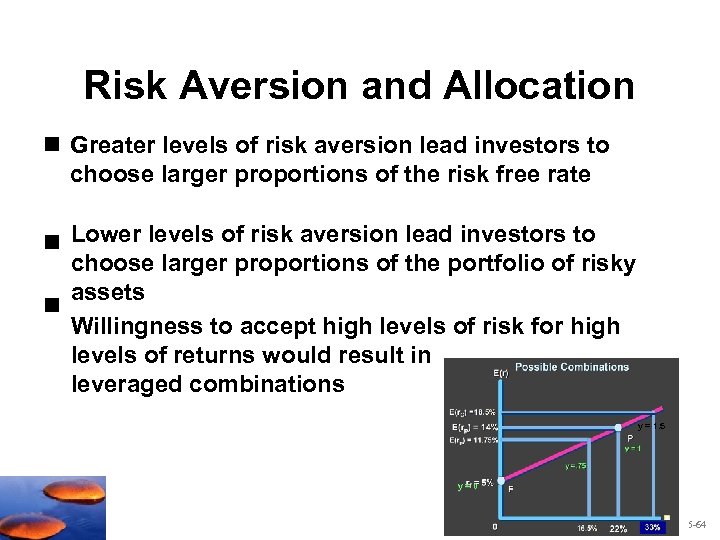Risk Aversion and Allocation n Greater levels of risk aversion lead investors to choose larger proportions of the risk free rate n Lower levels of risk aversion lead investors to choose larger proportions of the portfolio of risky assets n Willingness to accept high levels of risk for high levels of returns would result in leveraged combinations y = 1. 5 y=0 5 -64

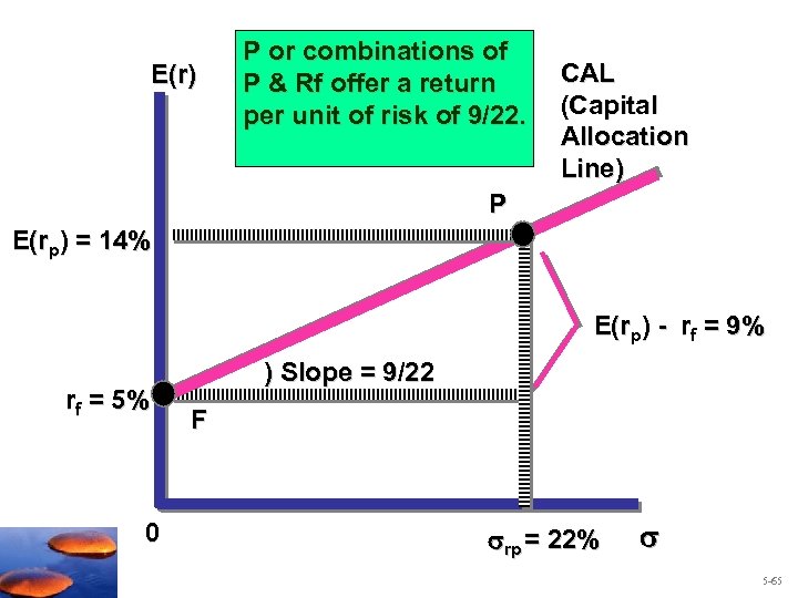E(r) P or combinations of P & Rf offer a return per unit of risk of 9/22. CAL (Capital Allocation Line) P E(rp) = 14% E(rp) - rf = 9% rf = 5% 0 ) Slope = 9/22 F rp = 22% 5 -65

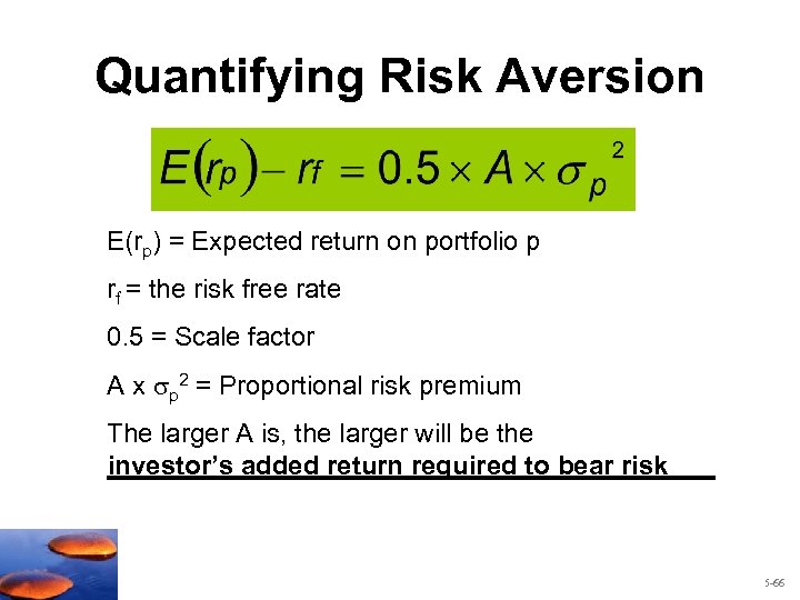Quantifying Risk Aversion E(rp) = Expected return on portfolio p rf = the risk free rate 0. 5 = Scale factor A x p 2 = Proportional risk premium The larger A is, the larger will be the _____________________ investor’s added return required to bear risk 5 -66

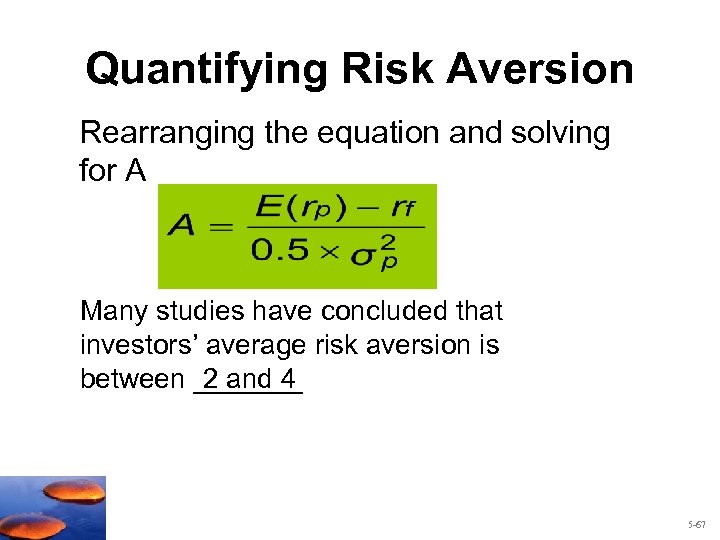Quantifying Risk Aversion Rearranging the equation and solving for A Many studies have concluded that investors’ average risk aversion is between _______ 2 and 4 5 -67

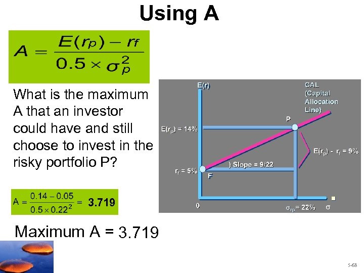Using A What is the maximum A that an investor could have and still choose to invest in the risky portfolio P? 3. 719 Maximum A = 3. 719 5 -68

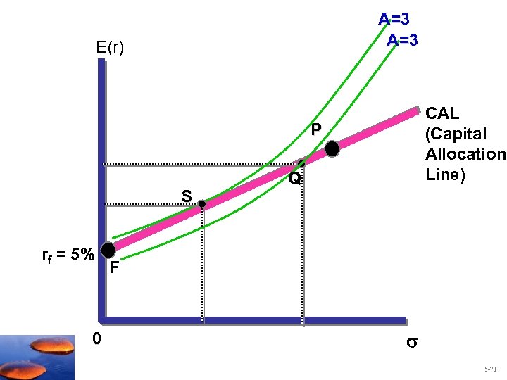
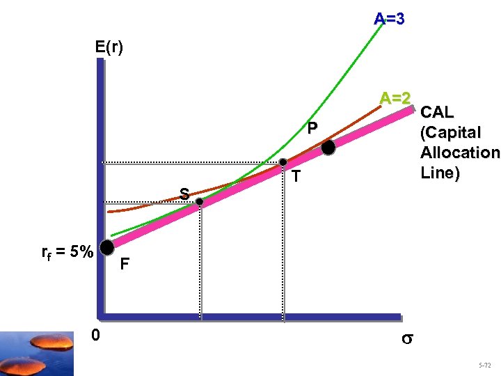
“A” and Indifference Curves § The A term can used to create indifference curves. § Indifference curves describe different combinations of return and risk that provide equal utility (U) or satisfaction. § U = E[r] - 1/2 A p 2 § Indifference curves are curvilinear because they exhibit diminishing marginal utility of wealth. • The greater the A the steeper the indifference curve and all else equal, such investors will invest less in risky assets. • The smaller the A the flatter the indifference curve and all else equal, such investors will invest more in risky assets. 5 -69

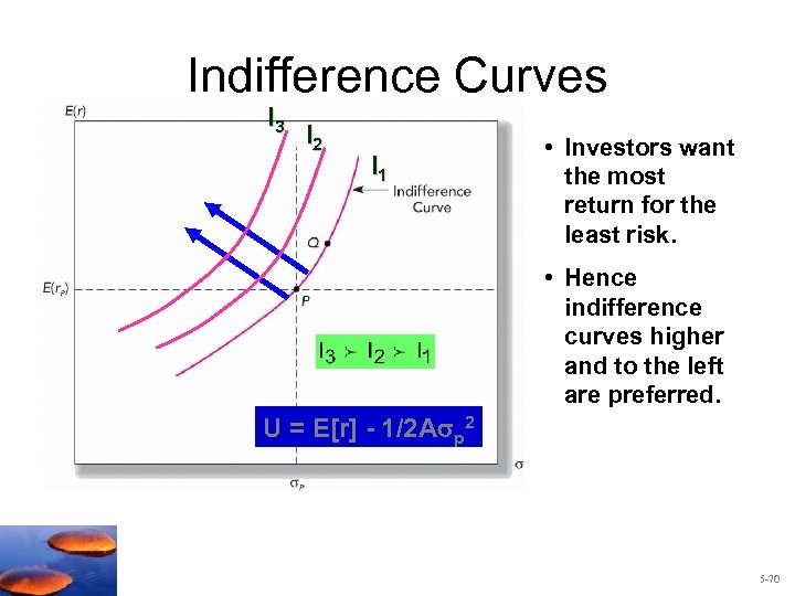Indifference Curves I 3 I 2 I 1 • Investors want the most return for the least risk. • Hence indifference curves higher and to the left are preferred. U = E[r] - 1/2 A p 2 5 -70

A=3 E(r) CAL (Capital Allocation Line) P S rf = 5% 0 Q F 5 -71

A=3 E(r) A=2 P S rf = 5% 0 T CAL (Capital Allocation Line) F 5 -72

5. 6 Passive Strategies and the Capital Market Line 5 -73

A Passive Strategy • Investing in a broad stock index and a risk free investment is an example of a passive strategy. – The investor makes no attempt to actively find undervalued strategies nor actively switch their asset allocations. – The CAL that employs the market (or an index that mimics overall market performance) is called the Capital Market Line or CML. 5 -74

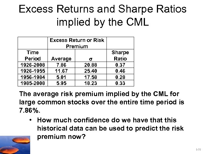Excess Returns and Sharpe Ratios implied by the CML Excess Return or Risk Premium Time Period 1926 -2008 1926 -1955 1956 -1984 1985 -2008 Average 7. 86 11. 67 5. 01 5. 95 20. 88 25. 40 17. 58 18. 23 Sharpe Ratio 0. 37 0. 46 0. 28 0. 33 The average risk premium implied by the CML for large common stocks over the entire time period is 7. 86%. • How much confidence do we have that this historical data can be used to predict the risk premium now? 5 -75

Active versus Passive Strategies • Active strategies entail more trading costs than passive strategies. • Passive investor “free-rides” in a competitive investment environment. • Passive involves investment in two passive portfolios – Short-term T-bills – Fund of common stocks that mimics a broad market index – Vary combinations according to investor’s risk aversion. 5 -76

Selected Problems 5 -77

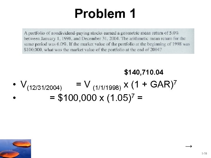Problem 1 $140, 710. 04 • V(12/31/2004) = V (1/1/1998) x (1 + GAR)7 • = $100, 000 x (1. 05)7 = → 5 -78

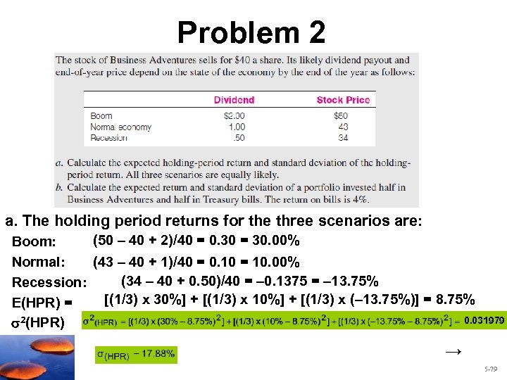Problem 2 a. The holding period returns for the three scenarios are: (50 – 40 + 2)/40 = 0. 30 = 30. 00% Boom: Normal: (43 – 40 + 1)/40 = 0. 10 = 10. 00% (34 – 40 + 0. 50)/40 = – 0. 1375 = – 13. 75% Recession: [(1/3) x 30%] + [(1/3) x 10%] + [(1/3) x (– 13. 75%)] = 8. 75% E(HPR) = 0. 031979 2(HPR) → 5 -79

Problem 2 Cont. Risky E[rp] = 8. 75% Risky p = 17. 88% b. E(r) = (0. 5 x 8. 75%) + (0. 5 x 4%) = 6. 375% = 0. 5 x 17. 88% = 8. 94% → 5 -80

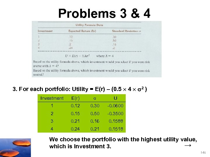Problems 3 & 4 3. For each portfolio: Utility = E(r) – (0. 5 4 2 ) Investment E(r) U 1 0. 12 0. 30 -0. 0600 2 0. 15 0. 50 -0. 3500 3 0. 21 0. 16 0. 1588 4 0. 21 0. 1518 We choose the portfolio with the highest utility value, → which is Investment 3. 5 -81

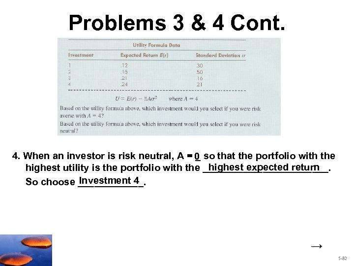Problems 3 & 4 Cont. 4. When an investor is risk neutral, A = 0 so that the portfolio with the _ highest expected return highest utility is the portfolio with the ____________. Investment 4 So choose ______. → 5 -82

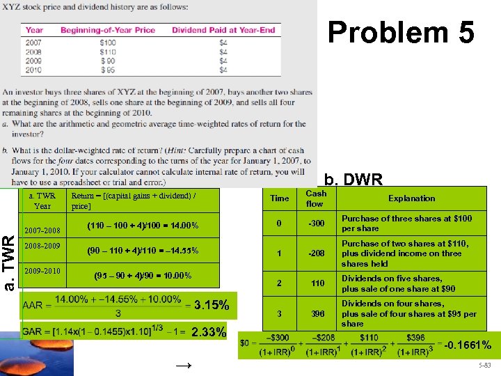a. TWR Problem 5 b. DWR a. TWR Year 2007 -2008 -2009 -2010 (110 – 100 + 4)/100 = 14. 00% (90 – 110 + 4)/110 = – 14. 55% (95 – 90 + 4)/90 = 10. 00% 3. 15% 2. 33% → Time Cash flow 0 -300 Purchase of three shares at $100 per share 1 -208 Purchase of two shares at $110, plus dividend income on three shares held 2 Return = [(capital gains + dividend) / price] 110 Dividends on five shares, plus sale of one share at $90 3 396 Dividends on four shares, plus sale of four shares at $95 per share Explanation -0. 1661% 5 -83