Chapter 5 Present Worth Analysis 1 What

Chapter 5 Present Worth Analysis 1

What have we learnt so far? We have learnt how to manipulate cash flows to solve compound interest problems. This only sets the stage for the main topic of the following chapters – Solving Economic Analysis problems. 2

Assumptions used in our analysis The trick is to use simplifying assumptions without compromising the applicability of the solution to real life. Six assumptions will be used 1. End-of-year convention 2. Viewpoint of Economic Analysis 3. Sunk costs 4. Borrowed money viewpoint 5. Effect of inflation and deflation 6. Income taxes 3

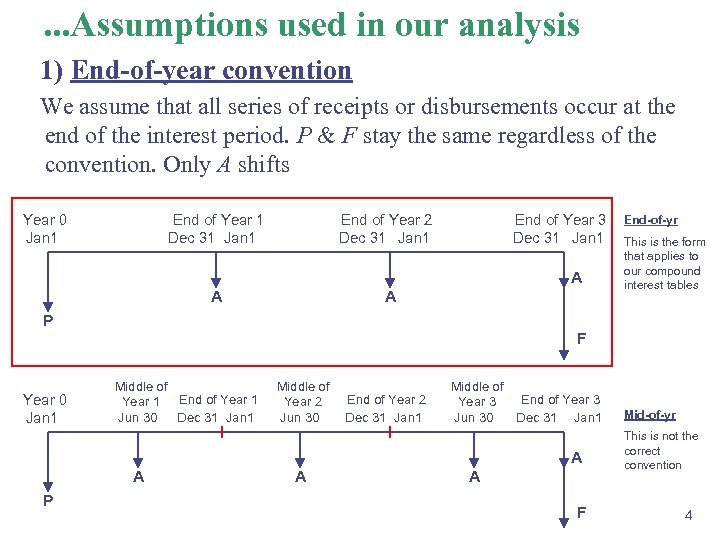. . . Assumptions used in our analysis 1) End-of-year convention We assume that all series of receipts or disbursements occur at the end of the interest period. P & F stay the same regardless of the convention. Only A shifts Year 0 Jan 1 End of Year 1 Dec 31 Jan 1 End of Year 2 Dec 31 Jan 1 End of Year 3 Dec 31 Jan 1 A A A End-of-yr This is the form that applies to our compound interest tables P F Year 0 Jan 1 Middle of Year 1 End of Year 1 Jun 30 Dec 31 Jan 1 Middle of End of Year 2 Jun 30 Dec 31 Jan 1 Middle of End of Year 3 Jun 30 Dec 31 Jan 1 A A P A A F Mid-of-yr This is not the correct convention 4

. . . Assumptions used in our analysis 2) Viewpoint of Economic Analysis Studies Take the point of view of a total firm. Don’t select a narrow viewpoint. (See example 1 -1 in your text) 3) Sunk Costs Only current and future differences between alternatives should be considered. Therefore, sunk costs should be disregarded. 4) Borrowed Money Viewpoint Two aspects of money to determine: 1. Financing (the problem of obtaining the money) 2. Investment (the problem of spending the money) These two aspects should be distinguished and separated. The money required to finance alternatives in problem solving is considered to be borrowed at interest rate i. 5

. . . Assumptions used in our analysis 5) Effect of Inflation and Deflation Our assumption is that prices are stable (Not inflation or deflation). This means that a machine the costs $5000 today can be expected to cost the same amount several years hence. 6) Income Taxes For now, we will not consider income taxes in our economic analysis. 6

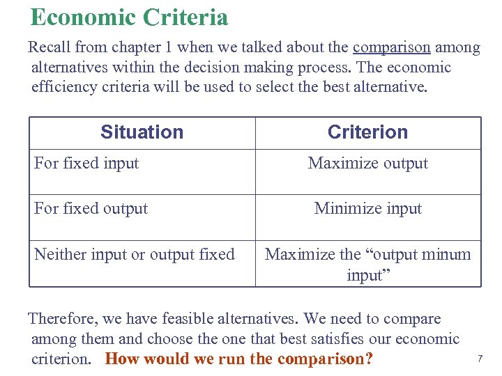Economic Criteria Recall from chapter 1 when we talked about the comparison among alternatives within the decision making process. The economic efficiency criteria will be used to select the best alternative. Situation Criterion For fixed input Maximize output For fixed output Minimize input Neither input or output fixed Maximize the “output minum input” Therefore, we have feasible alternatives. We need to compare among them and choose the one that best satisfies our economic criterion. How would we run the comparison? 7

Compare among Alternatives Due to time value of money, we will use the logic of equivalence to be able to run a fair comparison and make a sound decision. Three main methods of comparison 1. Present worth analysis (chapter 5) • Alternatives are converted into equivalent present consequences 2. Anuual cash flow analysis (chapter 6) • Alternatives are converted into equivalent uniform annual cash flow 3. Rate of return analysis (chapter 7) • Solve for the interest rate at which favorable consequences – that is benefits – are equivalent to unfavorable consequences – or costs. All of these methods are exact methods that will yield the same solution. So, choose the easier method. 8

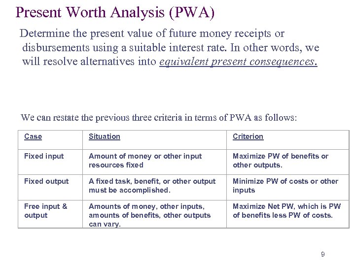Present Worth Analysis (PWA) Determine the present value of future money receipts or disbursements using a suitable interest rate. In other words, we will resolve alternatives into equivalent present consequences. We can restate the previous three criteria in terms of PWA as follows: Case Situation Fixed input Amount of money or other input resources fixed Fixed output A fixed task, benefit, or other output must be accomplished. Free input & output Amounts of money, other inputs, amounts of benefits, other outputs can vary. Criterion Maximize PW of benefits or other outputs. Minimize PW of costs or other inputs Maximize Net PW, which is PW of benefits less PW of costs. 9

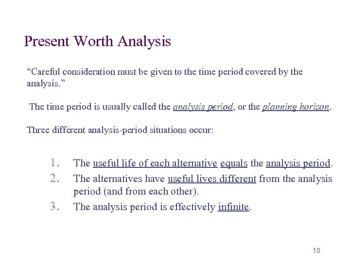Present Worth Analysis “Careful consideration must be given to the time period covered by the analysis. ” The time period is usually called the analysis period, or the planning horizon. Three different analysis-period situations occur: 1. 2. 3. The useful life of each alternative equals the analysis period. The alternatives have useful lives different from the analysis period (and from each other). The analysis period is effectively infinite. 10

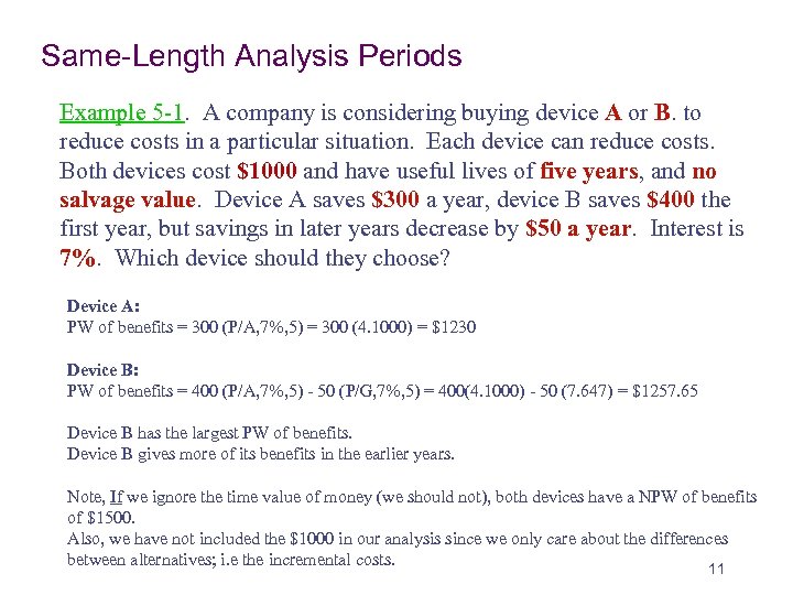Same-Length Analysis Periods Example 5 -1. A company is considering buying device A or B. to reduce costs in a particular situation. Each device can reduce costs. Both devices cost $1000 and have useful lives of five years, and no salvage value. Device A saves $300 a year, device B saves $400 the first year, but savings in later years decrease by $50 a year. Interest is 7%. Which device should they choose? Device A: PW of benefits = 300 (P/A, 7%, 5) = 300 (4. 1000) = $1230 Device B: PW of benefits = 400 (P/A, 7%, 5) - 50 (P/G, 7%, 5) = 400(4. 1000) - 50 (7. 647) = $1257. 65 Device B has the largest PW of benefits. Device B gives more of its benefits in the earlier years. Note, If we ignore the time value of money (we should not), both devices have a NPW of benefits of $1500. Also, we have not included the $1000 in our analysis since we only care about the differences between alternatives; i. e the incremental costs. 11

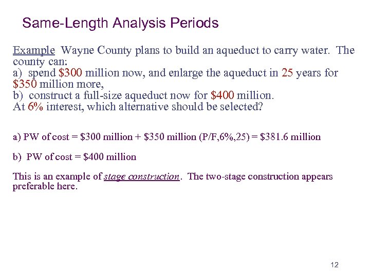Same-Length Analysis Periods Example Wayne County plans to build an aqueduct to carry water. The county can: a) spend $300 million now, and enlarge the aqueduct in 25 years for $350 million more, b) construct a full-size aqueduct now for $400 million. At 6% interest, which alternative should be selected? a) PW of cost = $300 million + $350 million (P/F, 6%, 25) = $381. 6 million b) PW of cost = $400 million This is an example of stage construction. The two-stage construction appears preferable here. 12

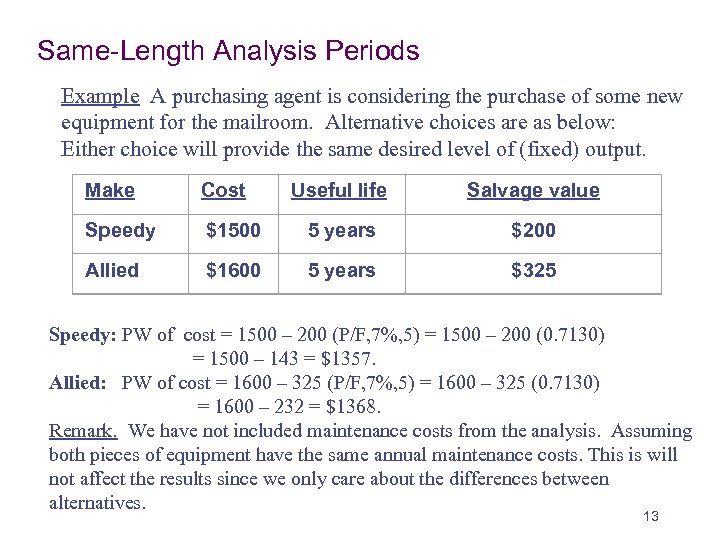Same-Length Analysis Periods Example A purchasing agent is considering the purchase of some new equipment for the mailroom. Alternative choices are as below: Either choice will provide the same desired level of (fixed) output. Make Cost Useful life Salvage value Speedy $1500 5 years $200 Allied $1600 5 years $325 Speedy: PW of cost = 1500 – 200 (P/F, 7%, 5) = 1500 – 200 (0. 7130) = 1500 – 143 = $1357. Allied: PW of cost = 1600 – 325 (P/F, 7%, 5) = 1600 – 325 (0. 7130) = 1600 – 232 = $1368. Remark. We have not included maintenance costs from the analysis. Assuming both pieces of equipment have the same annual maintenance costs. This is will not affect the results since we only care about the differences between alternatives. 13

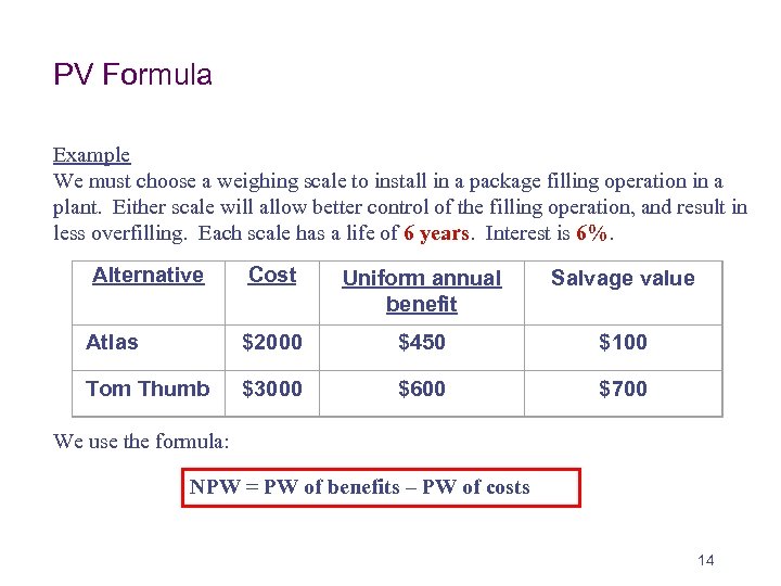PV Formula Example We must choose a weighing scale to install in a package filling operation in a plant. Either scale will allow better control of the filling operation, and result in less overfilling. Each scale has a life of 6 years. Interest is 6%. Alternative Cost Uniform annual Salvage value benefit Atlas $450 $100 Tom Thumb $2000 $3000 $600 $700 We use the formula: NPW = PW of benefits – PW of costs 14

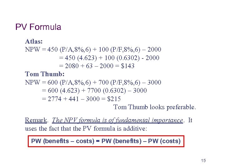PV Formula Atlas: NPW = 450 (P/A, 8%, 6) + 100 (P/F, 8%, 6) – 2000 = 450 (4. 623) + 100 (0. 6302) - 2000 = 2080 + 63 – 2000 = $143 Tom Thumb: NPW = 600 (P/A, 8%, 6) + 700 (P/F, 8%, 6) – 3000 = 600 (4. 623) + 7700 (0. 6302) – 3000 = 2774 + 441 – 3000 = $215 Tom Thumb looks preferable. Remark. The NPV formula is of fundamental importance. It uses the fact that the PV formula is additive: PW (benefits – costs) = PW (benefits) – PW (costs) 15

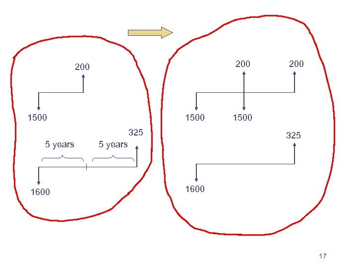
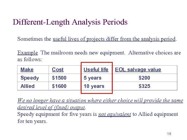Different-Length Analysis Periods Sometimes the useful lives of projects differ from the analysis period. Example The mailroom needs new equipment. Alternative choices are as follows: Make Cost Useful life EOL salvage value Speedy $1500 5 years $200 Allied $1600 10 years $325 We no longer have a situation where either choice will provide the same desired level of (fixed) output. Speedy equipment for five years is not equivalent to Allied equipment for ten years. 16

200 1500 325 5 years 1600 17

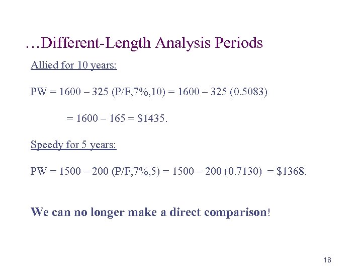…Different-Length Analysis Periods Allied for 10 years: PW = 1600 – 325 (P/F, 7%, 10) = 1600 – 325 (0. 5083) = 1600 – 165 = $1435. Speedy for 5 years: PW = 1500 – 200 (P/F, 7%, 5) = 1500 – 200 (0. 7130) = $1368. We can no longer make a direct comparison! 18

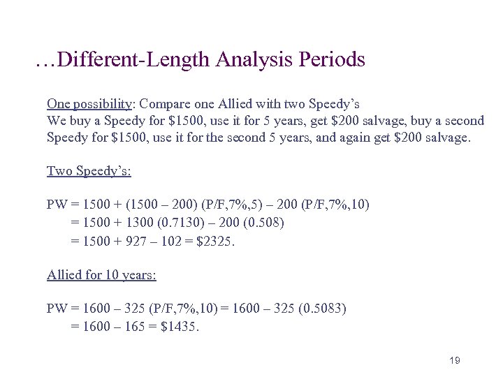…Different-Length Analysis Periods One possibility: Compare one Allied with two Speedy’s We buy a Speedy for $1500, use it for 5 years, get $200 salvage, buy a second Speedy for $1500, use it for the second 5 years, and again get $200 salvage. Two Speedy’s: PW = 1500 + (1500 – 200) (P/F, 7%, 5) – 200 (P/F, 7%, 10) = 1500 + 1300 (0. 7130) – 200 (0. 508) = 1500 + 927 – 102 = $2325. Allied for 10 years: PW = 1600 – 325 (P/F, 7%, 10) = 1600 – 325 (0. 5083) = 1600 – 165 = $1435. 19

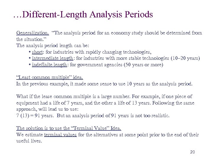…Different-Length Analysis Periods Generalization. “The analysis period for an economy study should be determined from the situation. ” The analysis period length can be: • short: for industries with rapidly changing technologies, • intermediate length: for industries with more stable technologies (10– 20 years) • indefinite length: for government agencies (50 years or more) “Least common multiple” idea. In the previous example, it made some sense to use 10 years as the analysis period. What if the lease common multiple is a large number. For example, if one piece of equipment had a life of 7 years, and the other a life of 13 years. Following the same approach, will lead us to use: 7 (13) = 91 years. But an analysis period of 91 years is not too realistic. The solution is to use the “Terminal Value” Idea. We estimate terminal values for the alternatives at some point prior to the end of their useful lives. 20

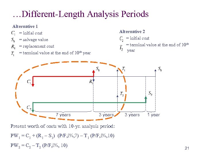…Different-Length Analysis Periods Alternative 1 = initial cost = salvage value = replacement cost = terminal value at the end of 10 th year 7 years Alternative 2 = initial cost = terminal value at the end of 10 th year 3 years 1 year Present worth of costs with 10 -yr. analysis period: PW 1 = C 1 + (R 1 – S 1) (P/F, i%, 7) – T 1 (P/F, i%, 10) PW 2 = C 2 – T 2 (P/F, i%, 10) 21

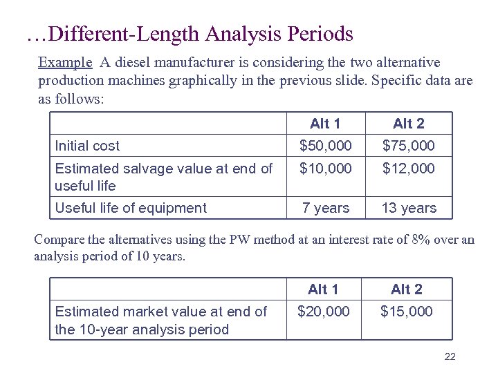…Different-Length Analysis Periods Example A diesel manufacturer is considering the two alternative production machines graphically in the previous slide. Specific data are as follows: Alt 1 Alt 2 Initial cost $50, 000 $75, 000 Estimated salvage value at end of useful life $10, 000 $12, 000 Useful life of equipment 7 years 13 years Compare the alternatives using the PW method at an interest rate of 8% over an analysis period of 10 years. Alt 1 Estimated market value at end of the 10 -year analysis period Alt 2 $20, 000 $15, 000 22

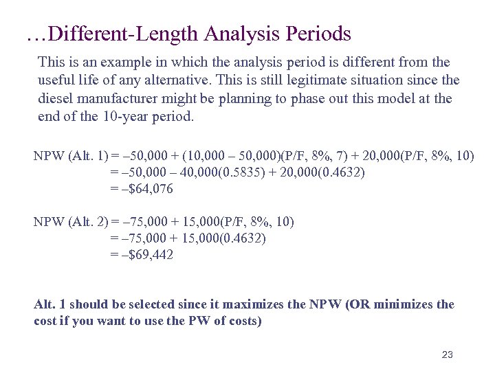…Different-Length Analysis Periods This is an example in which the analysis period is different from the useful life of any alternative. This is still legitimate situation since the diesel manufacturer might be planning to phase out this model at the end of the 10 -year period. NPW (Alt. 1) = – 50, 000 + (10, 000 – 50, 000)(P/F, 8%, 7) + 20, 000(P/F, 8%, 10) = – 50, 000 – 40, 000(0. 5835) + 20, 000(0. 4632) = –$64, 076 NPW (Alt. 2) = – 75, 000 + 15, 000(P/F, 8%, 10) = – 75, 000 + 15, 000(0. 4632) = –$69, 442 Alt. 1 should be selected since it maximizes the NPW (OR minimizes the cost if you want to use the PW of costs) 23

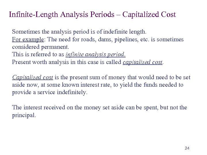Infinite-Length Analysis Periods – Capitalized Cost Sometimes the analysis period is of indefinite length. For example: The need for roads, dams, pipelines, etc. is sometimes considered permanent. This is referred to as infinite analysis period. Present worth analysis in this case is called capitalized cost. Capitalized cost is the present sum of money that would need to be set aside now, at some known interest rate, to yield the funds needed to provide a service indefinitely. The interest received on the money set aside can be spent, but not the principal. 24

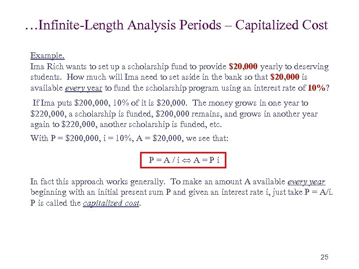…Infinite-Length Analysis Periods – Capitalized Cost Example. Ima Rich wants to set up a scholarship fund to provide $20, 000 yearly to deserving students. How much will Ima need to set aside in the bank so that $20, 000 is available every year to fund the scholarship program using an interest rate of 10%? If Ima puts $200, 000, 10% of it is $20, 000. The money grows in one year to $220, 000, a scholarship is funded, $200, 000 remains, and grows in another year again to $220, 000, another scholarship is funded, etc. With P = $200, 000, i = 10%, A = $20, 000, we see that: P = A / i A = P i In fact this approach works generally. To make an amount A available every year beginning with an initial present sum P and given an interest rate i, just take P = A/i. P is called the capitalized cost. 25

…Infinite-Length Analysis Periods – Capitalized Cost Example. How much should one set aside to pay $50 per year for maintenance on a gravesite if interest is assumed to be 4%? For perpetual maintenance, the principal sum must remain undiminished after making the annual disbursement. Capital cost P = A/i = 50/0. 04 = $1250 Therefore, one should set aside the amount of $1250 in order to keep paying $50 for the maintenance. 26

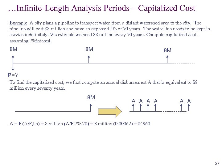…Infinite-Length Analysis Periods – Capitalized Cost Example A city plans a pipeline to transport water from a distant watershed area to the city. The pipeline will cost $8 million and have an expected life of 70 years. The water line needs to be kept in service indefinitely. We estimate we need $8 million every 70 years. Compute capitalized cost , assuming 7%interest. 8 M 8 M 8 M P=? To find the capitalized cost, we first compute an annual disbursement A that is equivalent to $8 million every seventy years. 8 M A A A A = F (A/F, i, n) = 8 million (A/F, 7%, 70) = 8 million (0. 00062) = $4960 27

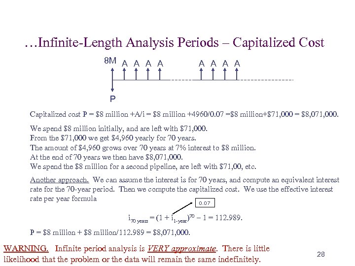…Infinite-Length Analysis Periods – Capitalized Cost 8 M A A A A P Capitalized cost P = $8 million +A/i = $8 million +4960/0. 07 =$8 million+$71, 000 = $8, 071, 000. We spend $8 million initially, and are left with $71, 000. From the $71, 000 we get $4, 960 yearly for 70 years. The amount of $4, 960 grows over 70 years at 7% interest to $8 million. At the end of 70 years we then have $8, 071, 000. We spend the $8 million for a second pipeline, are left with $71, 00, etc. Another approach. We can assume the interest is for 70 years, and compute an equivalent interest rate for the 70 -year period. Then we compute the capitalized cost. We use the effective interest rate per year formula 0. 07 i 70 years = (1 + i 1 -year)70 – 1 = 112. 989. P = $8 million + $8 million/112. 989 = $8, 071, 000. WARNING. Infinite period analysis is VERY approximate. There is little likelihood that the problem or the data will remain the same indefinitely. 28

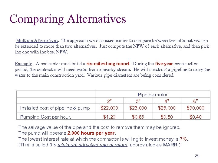Comparing Alternatives Multiple Alternatives. The approach we discussed earlier to compare between two alternatives can be extended to more than two alternatives. Just compute the NPW of each alternative, and then pick the one with the best NPW. Example A contractor must build a six-miles-long tunnel. During the five-year construction period, the contractor will need water from a nearby stream. He will construct a pipeline to carry the water to the main construction yard. Various pipe diameters are being considered. Installed cost of pipeline & pump Pumping Cost per hour. 2” $22, 000 $1. 20 Pipe diameter 3” 4” $23, 000 $25, 000 $0. 65 $0. 50 6” $30, 000 $0. 40 The salvage value of the pipe and the cost to remove them may be ignored. The pump will operate 2, 000 hours per year. The lowest interest rate at which the contractor is willing to invest money is 7%. (This is called the minimum attractive rate of return, abbreviated as MARR. ) 29

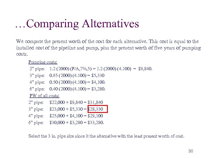…Comparing Alternatives We compute the present worth of the cost for each alternative. This cost is equal to the installed cost of the pipeline and pump, plus the present worth of five years of pumping costs. Pumping costs: 2” pipe: 1. 2 (2000) (P/A, 7%, 5) = 1. 2 (2000) (4. 100) = $9, 840. 3” pipe: 0. 65 (2000) (4. 100) = $5, 330 4” pipe: 0. 50 (2000) (4. 100) = $4, 100. 6” pipe: 0. 40 (2000) (4. 100) = $3, 280. PW of all costs: 2” pipe: $22, 000 + $9, 840 = $31, 840 3” pipe: $23, 000 + $5, 330 = $28, 330 4” pipe: $25, 000 + $4, 100 = $29, 100 6” pipe: $30, 000 + $3, 280 = $33, 280. Select the 3 in. pipe size since it the alternative with the least present worth of cost. 30

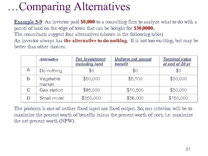…Comparing Alternatives Example 5 -9 An investor paid $8, 000 to a consulting firm to analyze what to do with a parcel of land on the edge of town that can be bought for $30, 0000. The consultants suggest four alternatives (shown in the following table) An investor always has the alternative to do nothing. It is not too exciting, but may be better than other choices. Alternative Tot. Investment including land Uniform net annual benefit Terminal value at end of 20 yr A Do nothing $0 $0 $0 B $50, 000 $5, 100 $30, 000 C Vegetable market Gas station $95, 000 $10, 500 $30, 000 D Small motel $350, 000 $36, 000 $150, 000 The problem is one of neither fixed input nor fixed output. So, our criterion will be to maximize the present worth of benefits minus the present worth of cost; i. e. maximize the net present worth (NPW) 31

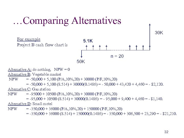…Comparing Alternatives 30 K For example Project B cash flow chart is 5. 1 K n = 20 50 K Alternative A: do nothing, NPW = 0 Alternative B: Vegetable market NPW = -50, 000 + 5, 100 (P/A, 10%, 20) + 30000 (P/F, 10%, 20) = -50, 000 + 5, 100 (8. 514) + 30000(0. 1486) = - 50, 000 + 43, 420 + 4, 460 = - $2, 120. Alternative C: Gas station NPW = -95000 + 10500 (P/A, 10%, 20) + 30000 (P/F, 10%, 20) = -95, 000 + 10500 (8. 514) + 30000(0. 1486) = - 95, 000 + 9, 400 + 4, 460 = - $1, 140. Alternative D: Small motel NPW = -350, 000 + 36000 (P/A, 10%, 20) + 150000 (P/F, 10%, 20) = -350, 000 + 36000 (8. 514) + 150000(0. 1486) = - 350, 000 + 306, 500 + 23, 290 = - $21, 210. In this case it is best to do nothing. 32

…Comparing Alternatives Important note. The $8, 000 the investor spent for consulting services is a past cost, and is called a sunk cost. The only relevant costs in the economic analysis are present and future costs. Past events and past costs are gone and cannot be allowed to affect future planning. The authors do not mention it, but the sort of analysis the consultants did to provide the table was probably very approximate. Predicting the future is always very tricky. 33

…Comparing Alternatives Example 5 -10 Strip Mining. Land can be purchased for $610, 000 to be strip-mined for coal. Annual net income will be $200, 000 per year for ten years. At the end of the ten years, the surface of the land must be restored according to federal law. The cost of reclamation will be $1, 500, 000 in excess of the resale value of the land after it is restored. The interest rate is 10%. Determine whether the project is desirable NPW = – 610 + 200 (P/A, 10%, 10) – 1500 (P/F, 10%, 10) = – 610 + 200 (6. 145) + 1500 (0. 3855) = – 610 + 1229 – 578 = +$41 ($41, 000) The NPW is positive, so the answer is “yes”. 34

…Comparing Alternatives Example 5 -11 Two pieces of construction equipment are being considered Year Alt. A Alt. B 0 -$2000 -$1500 1 +1000 +700 2 +850 +300 3 +700 +300 4 +550 +300 5 +400 +300 6 +400 7 +400 +500 8 +400 +600 Based on 8% interest rate, which alternative should be selected? 35

36