Chapter 5 Neural Network Concepts and Paradigms

Chapter 5 Neural Network Concepts and Paradigms

Chapter 5 Outline • History • Key elements and terminology • Topologies • Adaptation methods • Recall dynamics • Comparisons of neural and non-neural methods

History of Neural Networks • How did they get their name? • The Age of Camelot • The Dark Age • The Renaissance • The Age of Neoconnectionism • The Age of Computational Intelligence

Why the name Neural Networks? • Important development done by biologists, physiologists and psychologists (PDP group) • But also important roots in analog computing and signal processing, so engineering heritage is significant • Widrow: “Massively parallel adaptive filters” • “Carbon-based” science may provide important insights for reverse engineering

The Age of Camelot • William James • Mc. Culloch and Pitts • Donald Hebb • Frank Rosenblatt • Widrow and Hoff

William James (1890) • American psychologist • James’ Elementary Principle: “When two elementary brain processes have been active together or in immediate succession, one of them, on re-occurring, tends to propagate its excitement to the other. ” • Also wrote of the concept that a neuron’s activity is a function of the sum of the inputs, with past history contributing to the interconnection weights

Mc. Culloch and Pitts (1943) Five physical assumptions: * The activity of a neuron is an all or none process * A certain fixed number of synapses must be excited within the period of latent addition in order to excite a neuron at any time, and this number is independent of previous activity and position on the neuron * The only significant delay within the nervous system is synaptic delay * The activity of any inhibitory synapse absolutely prevents excitation of the neuron at that time * The structure of the net does not change with time These assumptions describe the “Mc. Culloch-Pitts neuron

Mc. Culloch and Pitts, cont’d. In most neural networks, however, • Binary PEs are seldom used • There is no “fixed number of connections” that must be excited • There is generally no time delay associated with a connection to a PE • A single negative connection does not generally inhibit a PE’s activation • While a NN structure may not change, the weights change during training, and connections are sometimes pruned; new CI tools may routinely change network structure in the future

Mc. Culloch and Pitts, cont’d. So, why important? * Proved that networks of their neurons could represent any finite logical expression * Used a massively parallel architecture * Provided important foundation for further development

Donald Hebb (1948) • Postulated Hebbian weight updating: When cell A repeatedly helps fire B, A’s efficiency in helping to fire B is increased. • Made four major contributions: * Recognized that information is stored in the weight of the synapses * Postulated a learning rate that is proportional to the product of neuron activation values * Assumed weights are symmetric * Postulated a cell assembly theory: Repeated simultaneous activation of weakly-connected cell group results in a more strongly connected group

Frank Rosenblatt (late 1950 s) • Defined first computer implementation: the perceptron, which could classify patterns by modifying its connections • Attracted attention of engineers and physicists, using model of biological vision • Defined information storage as being “in connections or associations rather than topographic representations, ” and stated that recognition/behavior “makes use of these new pathways which have been created, automatically activating the appropriate response. ” • Defined both self-organizing and supervised learning mechanisms, and in sequential pattern recognition.

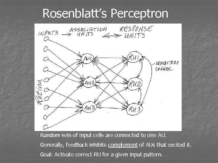Rosenblatt’s Perceptron Random sets of input cells are connected to one AU. Generally, feedback inhibits complement of AUs that excited it. Goal: Activate correct RU for a given input pattern.

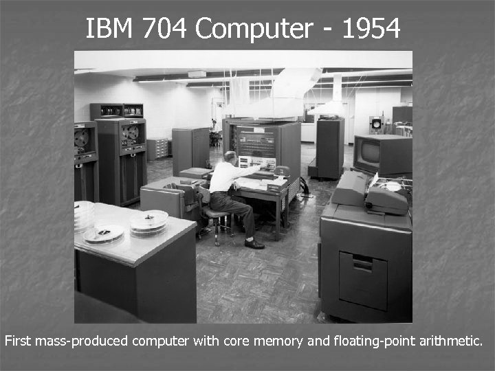IBM 704 Computer - 1954 First mass-produced computer with core memory and floating-point arithmetic.

Widrow and Hoff • Engineers (!) who simulated networks on computers and implemented designs in hardware (Adaline and Madaline) • Formulated Least Mean Squares (LMS) algorithm that minimizes sum-squared error: for n inputs, adjust each input to remove 1/n of the error. . . great speed improvement over perceptron • Early applications in telecommunications (echo elimination) and medicine (electrocardiogram analysis) • LMS adapts weights even when classifier output is correct

The Dark Age • Perceptrons • Stephen Grossberg • Shun-Ichi Amari • Teuvo Kohonen • Kunihiko Fukishima

Perceptrons • Minsky and Papert (1969) • Discusses two-layer perceptrons with threshold logic units • “. . . our intuitive judgement [is] that the extension [to multilayer perceptrons with hidden layers] is sterile. ” • Drove wedge between numerics and symbolics researchers • Neural network funding dried up

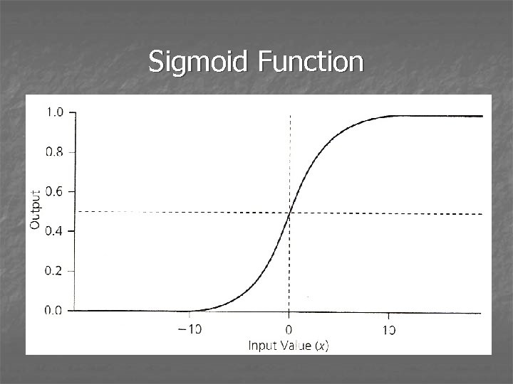
Stephen Grossberg • Work is abstract, theoretical and dense • Best known for Adaptive Resonance Theory • Developed “on-center off-surround” concept • Distinguished short-term (activation) and long-term (weights) memory; both with “forgetting” • Introduced sigmoid response functions for cell populations (non-negative, inhibitory) • Computed learning from sum of desired and actual outputs

Sigmoid Function

Shun-Ichi Amari • Developed error correction adaptation (learning) for hidden PEs • Analysis of randomly connected networks and temporarily associative memories • Developed concept of neuron pools, small mutually connected groups of neurons, as fundamental computing element • Recent important work in competitive learning and network memory capacity • Most current work in blind source separation (similar work to that of Prof. He Zhenya at Southeast University in China)

Teuvo Kohonen • Early work similar to James Anderson • Best known for the Self-organizing Feature Map (and its descendants), leading unsupervised adaptation technique • Introduced linear, continuous-valued PEs, connection weights and inputs • Networks with many simultaneously active input and output PEs (image and speech processing) • Activation patterns on multiple output PEs represent classifications

Kunihiko Fukishima • Best known for the neocognitron, a model for a visual pattern recognition mechanism • Complex: multiple layers of S-cells and C-cells; effect is to telescope input to output • Some translation and rotation invariance • Relatively complex structure (~10 K PEs andmultiple feedforward weight paths and feedback loops) • Developed way to teach “hidden” PEs in limited applications

The Renaissance • John Hopfield • The PDP Group * Hinton * Mc. Clelland * Rumelhart * Sejnowski *. . . 12 others

John Hopfield • 1982 paper helped revive the field • From physicist’s viewpoint: synthesized, generalized, proselytized, and pointed the way to implementation • Developed way to minimize “energy” of network, defined stable states • First NNs on silicon chips built by AT&T using Hopfield net

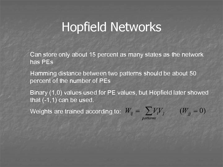Hopfield Networks Can store only about 15 percent as many states as the network has PEs Hamming distance between two patterns should be about 50 percent of the number of PEs Binary (1, 0) values used for PE values, but Hopfield later showed that (-1, 1) can be used. Weights are trained according to:

Hopfield Networks, Continued • The activation value of the PE is 1 if the net input is >= 0, -1 otherwise • In 1987, Bell Labs implemented Hopfield nets on silicon chips • Carver Mead at Cal Tech followed with VLSI nets for artificial retinas and cochleas

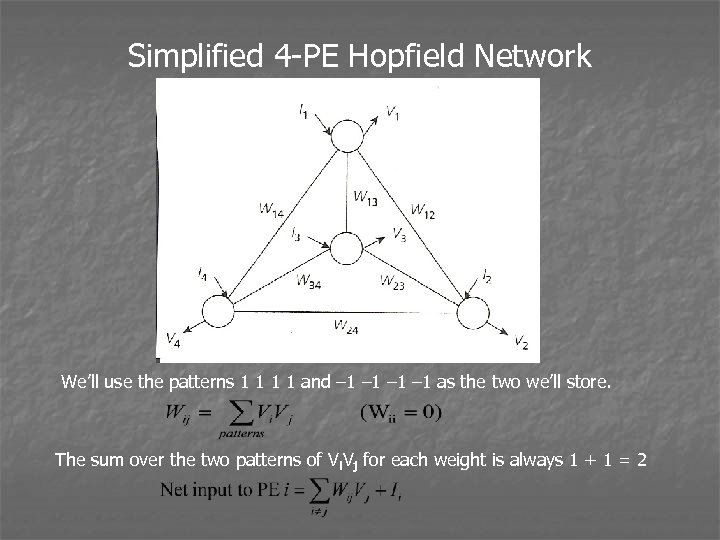Simplified 4 -PE Hopfield Network We’ll use the patterns 1 1 and – 1 – 1 as the two we’ll store. The sum over the two patterns of Vi. Vj for each weight is always 1 + 1 = 2

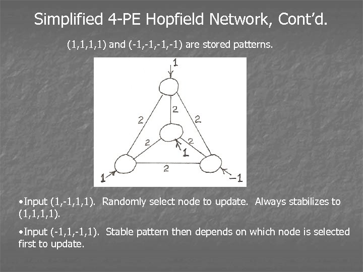Simplified 4 -PE Hopfield Network, Cont’d. (1, 1, 1, 1) and (-1, -1, -1) are stored patterns. • Input (1, -1, 1, 1). Randomly select node to update. Always stabilizes to (1, 1, 1, 1). • Input (-1, 1, -1, 1). Stable pattern then depends on which node is selected first to update.

According to Robert Hecht-Nielsen: … by the beginning of 1986, approximately onethird of the people in the field had been brought in directly by Hopfield or by one of his earlier converts. …

The Parallel Distributed Processing Group • Contributed to forming “critical mass” in neural network field • Published three volumes; most popular books in late 1980 s; synthesized all there was to know then • Vol. 1 Ch. 8 contains derivation of backpropagation algorithm • Introduced Boltzmann machines • Presented a variety of paradigms

The Age of Neoconnectionism 1987 -1998 • Donald Specht developed probabilistic neural networks • International leaders emerged, among them John Taylor (UK); Rolf Eckmiller (Germany); Toshio Fukuda (Japan); Paul Werbos, Richard Lippmann, Walter Freeman, Michael Arbib and Robert Marks (US); Sha Zong, Wu Youshou, and He Zhenya (China) • IEEE Neural Networks Council formed (now the IEEE Computational Intelligence Society); councils also formed in several countries/regions • Many network paradigms introduced, numerous applications developed • Use of personal computers (PCs) proliferated • First IEEE World Congress on Computational Intelligence in Orlando, Florida in 1994

The Age of Computational Intelligence 1998 -present • First use of the term (in its current context) by James Bezdek in 1992 • First text on CI in 1996 • As of 1997, IEEE Transactions in all three fields: neural networks, fuzzy systems, and evolutionary computation • Second IEEE World Congress on CI in Anchorage in 1998 • Neural Networks Society in 2002, Computational Intelligence Society in 2006. • Hybrid systems became common

Neural Network Theory and Paradigms • What are NNs and why are they useful? • NN components and terminology • NN topologies • NN learning • NN recall • NN taxonomy • Comparisons with other information processing methods

What NNs are and why they are useful • In the simplest terms, NNs map input vectors to output vectors • Operations performed include: * Classification * Pattern matching and completion * Noise removal * Optimization * Simulation * Control • NNs consist of processing elements (PEs) and weighted connections

What NNs are and why they are useful • Connection weights store the information • Weight values usually determined by adaptation procedure • Each PE acts independently of all others • Each PE relies only on local information • Connection pattern provides redundancy and facilitates fault tolerance • NNs are able to “learn” arbitrary non-linear mappings

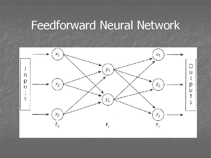Feedforward Neural Network

NNs are advantageous where: • Relatively few decisions are required from a massive amount of data • Nonlinear mappings must be automatically acquired • A near-optimal solution to a combinatorial optimization problem is required quickly

Principal elements required to specify NNs Topology - layers and interconnections Adaptation - how network is configured to store information Recall - How stored information is retrieved

Neural Network Components and Terminology • Input and output patterns • Weights • Processing elements • PE functions

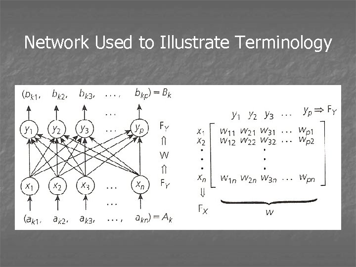Network Used to Illustrate Terminology

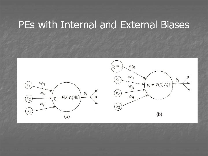
NN Components and Terminology IEEE Computational Intelligence Society Standards Committee Autoassociative - one pattern Heteroassociative - two patterns Weights provide the path and modulate the amount of signal passed between PEs Weights can be positive or negative Sparse connectivity means some weights have value of zero It is often desirable for PE to have a “bias” value

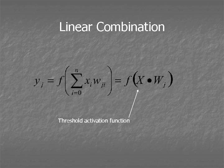
Processing Elements • Components of NNs where computations are performed • PEs have two important qualities: * They require only local information * They produce only one output value • Output of a PE is a function of the outputs of the previous layer and the weights from the PEs in that layer Actually, it’s a function of a function: calculate input to PE, then calculate PE output (activation)

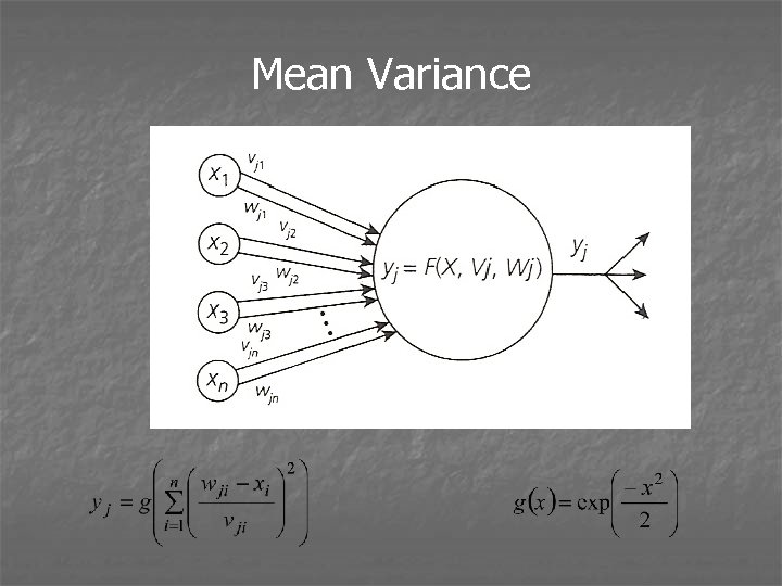
Examples of PE Input Calculations • Linear combination • Mean variance connections • Min-max connections • . . . others

PEs with Internal and External Biases

Input Computation Types n n Linear combination connections (most common) Mean-variance connections

Linear Combination Threshold activation function

The dot product is a similarity measure: For vectors of fixed length, maximizing dot product minimizes mean square separation:

Mean Variance

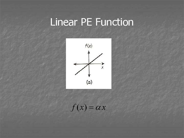
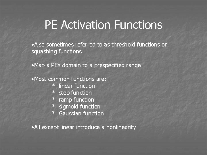PE Activation Functions • Also sometimes referred to as threshold functions or squashing functions • Map a PEs domain to a prespecified range • Most common functions are: * linear function * step function * ramp function * sigmoid function * Gaussian function • All except linear introduce a nonlinearity

Linear PE Function

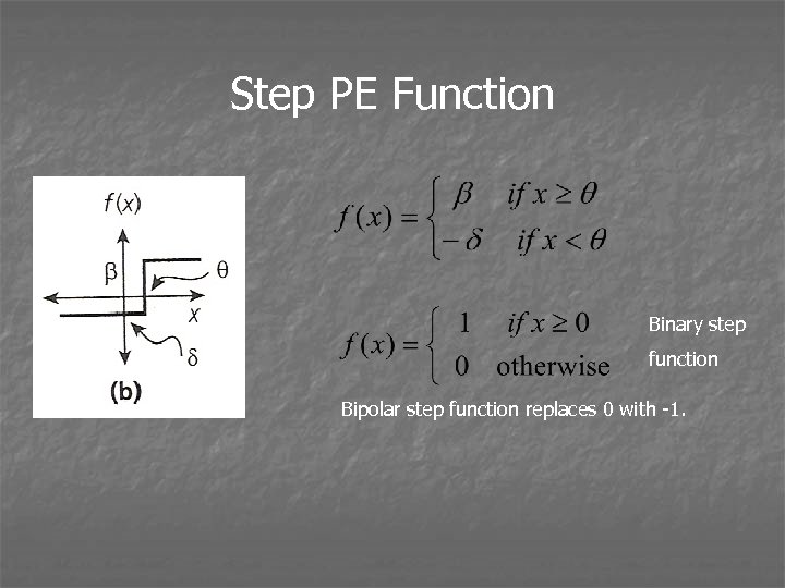Step PE Function Binary step function Bipolar step function replaces 0 with -1.

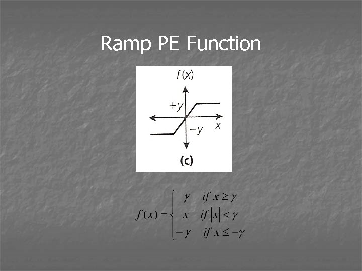Ramp PE Function

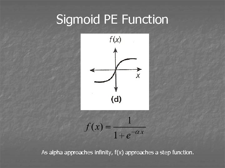Sigmoid PE Function As alpha approaches infinity, f(x) approaches a step function.

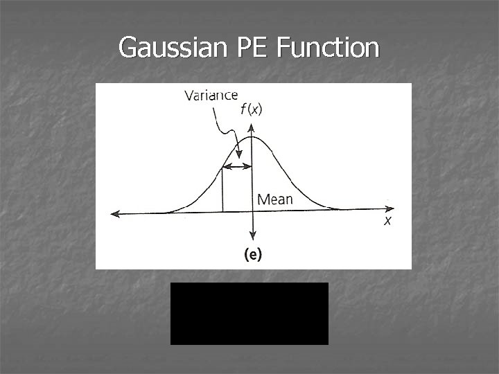Gaussian PE Function

Neural Network Topologies Topology: the arrangement of the PEs, connections and patterns into a NN

NN Topologies: Terminology Layers: All PEs in a layer have the same source(s) and destinations for weights, and same activation function Intralayer weights are between PEs in same layer; interlayer weights are between PEs in different layers Feedforward net feeds information in only one direction; if any feedback paths exist, it is a feedback (recurrent) NN

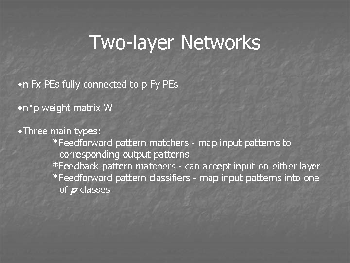Two-layer Networks • n Fx PEs fully connected to p Fy PEs • n*p weight matrix W • Three main types: *Feedforward pattern matchers - map input patterns to corresponding output patterns *Feedback pattern matchers - can accept input on either layer *Feedforward pattern classifiers - map input patterns into one of p classes

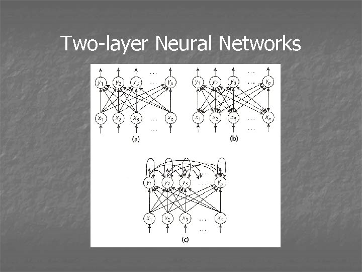Two-layer Neural Networks

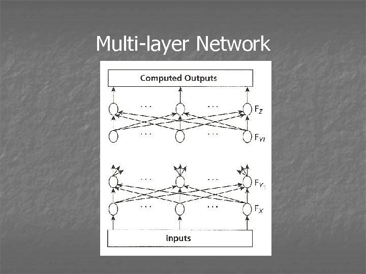
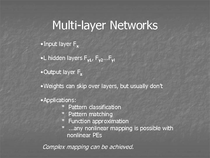Multi-layer Networks • Input layer Fx • L hidden layers Fy 1, Fy 2. . . Fyl • Output layer Fz • Weights can skip over layers, but usually don’t • Applications: * Pattern classification * Pattern matching * Function approximation *. . . any nonlinear mapping is possible with nonlinear PEs Complex mapping can be achieved.

Multi-layer Network

Multi-layer Networks: Issues • How many layers are sufficient? • How many PEs needed in (each) hidden layer? • How much data needed fro training?

Examples of Multi-layer NNs • Backpropagation • Neocognitron • Probabilistic NN (radial basis function NN) • Boltzmann machine • Cauchy machine • Radial basis function networks

Neural Network Adaptation • Adaptation (def. ) - Change in connection weight values that results in information capture that can be recalled later Sometimes referred to as “learning” • Supervised/unsupervised • Offline/online

Supervised Adaptation • Utilizes an external teacher and/or global information * Error correction adaptation * Hebbian adaptation * Competitive adaptation * Hardwired systems • Structural and temporal adaptation both used • Issues: * How long to train * How to measure results

Unsupervised Adaptation • Also called self-organization • No external teacher - relies on local information • Emergent collective properties are “discovered” • Examples: * Self-organizing feature maps * Competitive adaptation

Offline Adaptation • Used by most learning techniques • Training patterns used to condition weights prior to use; weights then frozen • All patterns must be present for training

On-line Adaptation • Add information real-time, non-destructively • Allows the network to learn in-situ • Examples: Adaptive Resonance Theory, fuzzy min-max

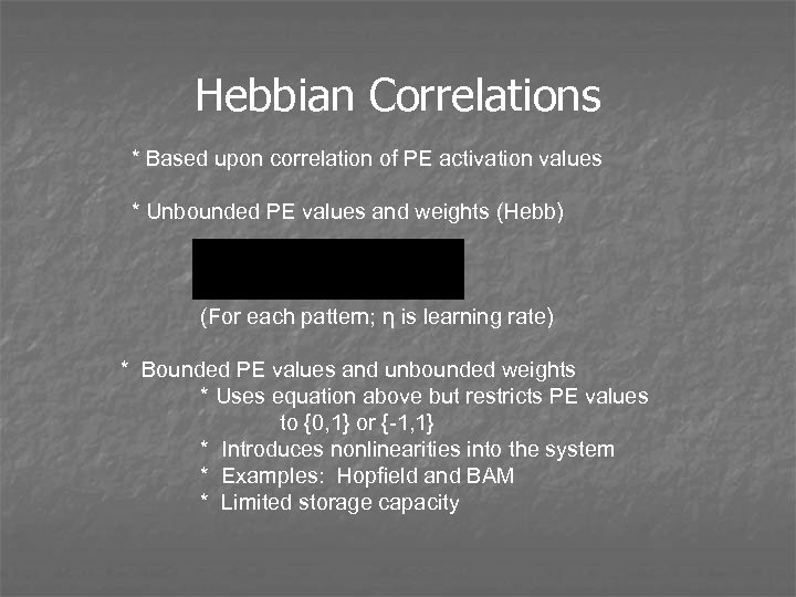Hebbian Correlations * Based upon correlation of PE activation values * Unbounded PE values and weights (Hebb) (For each pattern; η is learning rate) * Bounded PE values and unbounded weights * Uses equation above but restricts PE values to {0, 1} or {-1, 1} * Introduces nonlinearities into the system * Examples: Hopfield and BAM * Limited storage capacity

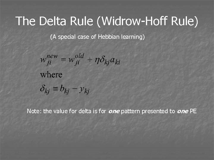The Delta Rule (Widrow-Hoff Rule) (A special case of Hebbian learning) Note: the value for delta is for one pattern presented to one PE

Competitive Adaptation • Automatically creates classes for a set of input patterns • Two-layer network • Two-step procedure • Couples recall process with learning process • Fx PEs encode input pattern, each Fy PE represents a class Researchers include: Grossberg Von der Malsburg Amari Takeuchi

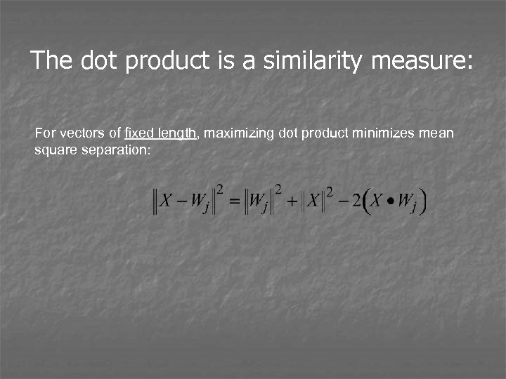
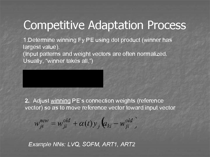Competitive Adaptation Process 1. Determine winning Fy PE using dot product (winner has largest value). (Input patterns and weight vectors are often normalized. Usually, “winner takes all. ”) 2. Adjust winning PE’s connection weights (reference vector) so as to move reference vector toward input vector Example NNs: LVQ, SOFM, ART 1, ART 2

Error Correction Adaptation • Weights are adjusted in proportion to difference between target and actual values of PE • Two-layer net limited to linear mappings • Multi-layer net can capture non-linear mappings

Multilayer Error Correction Adaptation Credit assignment problem: For how much of an output layer PE error is each hidden layer PE responsible? One key is to use a continuously differentiable activation function for hidden PEs.

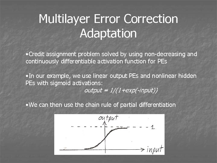Multilayer Error Correction Adaptation • Credit assignment problem solved by using non-decreasing and continuously differentiable activation function for PEs • In our example, we use linear output PEs and nonlinear hidden PEs with sigmoid activations: output = 1/(1+exp(-input)) • We can then use the chain rule of partial differentiation

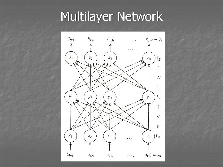Multilayer Network

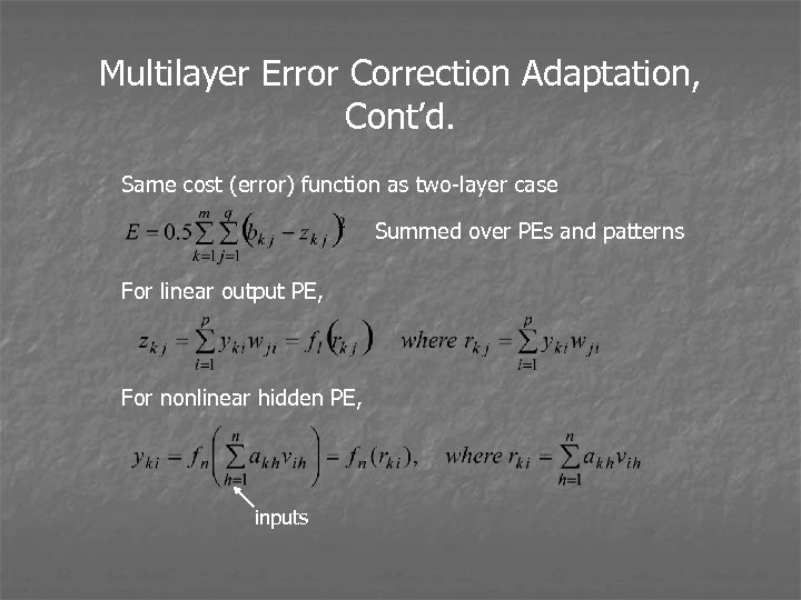Multilayer Error Correction Adaptation, Cont’d. Same cost (error) function as two-layer case Summed over PEs and patterns For linear output PE, For nonlinear hidden PE, inputs

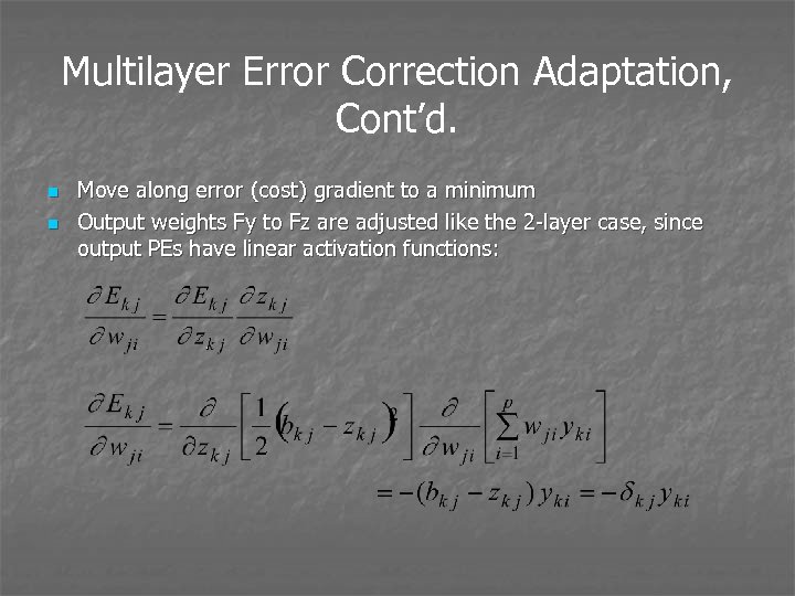Multilayer Error Correction Adaptation, Cont’d. n n Move along error (cost) gradient to a minimum Output weights Fy to Fz are adjusted like the 2 -layer case, since output PEs have linear activation functions:

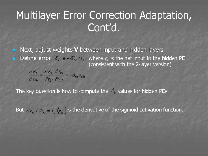Multilayer Error Correction Adaptation, Cont’d. n n Next, adjust weights V between input and hidden layers where rki is the net input to the hidden PE Define error (consistent with the 2 -layer version) The key question is how to compute the But values for hidden PEs is the derivative of the sigmoid activation function.

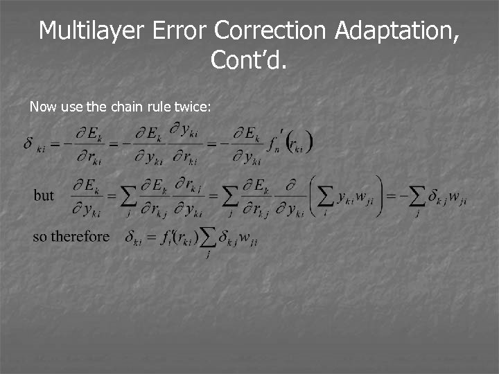Multilayer Error Correction Adaptation, Cont’d. Now use the chain rule twice:

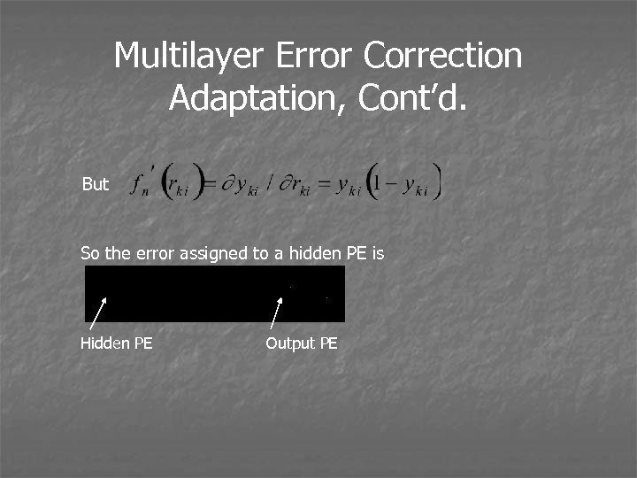Multilayer Error Correction Adaptation, Cont’d. But So the error assigned to a hidden PE is Hidden PE Output PE

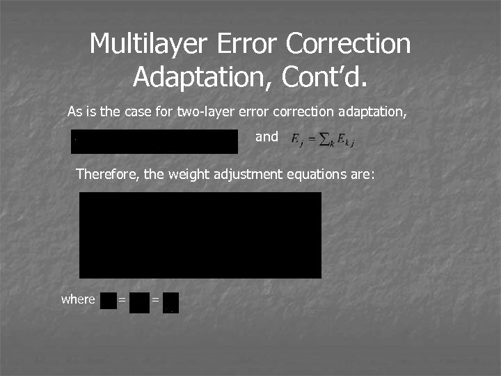Multilayer Error Correction Adaptation, Cont’d. As is the case for two-layer error correction adaptation, and Therefore, the weight adjustment equations are: where = =

Back-propagation Unresolved Issues • Number of training parameters • Number and configuration of hidden layer PEs • Avoidance of local minima during training • Relatively long training time

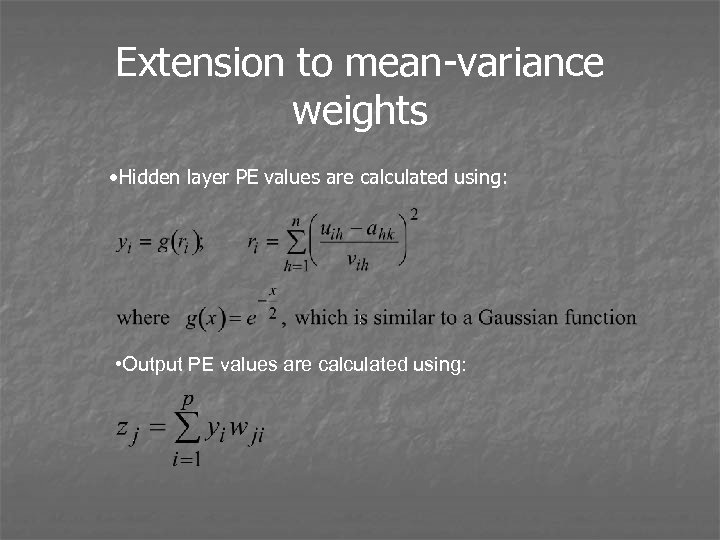Extension to mean-variance weights • Hidden layer PE values are calculated using: • Output PE values are calculated using:

Cluster Analysis, and Classification Cluster analysis: Assign patterns into one of several subgroups. Similar patterns are within same subgroup Differences between subgroups are maximized Classification: Each pattern is assigned to a class. Decision hypersurface is adjusted so as to minimize error.

Summary of Attributes Training time – Competitive adaptation is slow; back-propagation is very slow Off-line/on-line – Competitive adaptation either off- or on-line; backpropagation off-line only Supervised/unsupervised – Back-propagation supervised; competitive learning unsupervised Linear/nonlinear – Back-propagation is nonlinear; competitive learning linear only Storage capacity (with respect to the number of weights)- Competitive learning is fairly high; back-propagation is high

Other Information Processing Methods Stochastic Approximation - Same as 2 - and 3 -layer error correction algorithms Kalman Filters - Predict the next state of a system; often used for control systems. Back-propagation is a special case of extended Kalman filter algorithm Linear and Nonlinear Regression - 2 -layer error correction similar to linear regression; back-propagation is similar to non-linear regression (minimizing mean-square error is equivalent to curve fitting)

Other Info. Processing Methods, Cont’d. Correlation - Compares two patterns; uses dot product; similar to Hebbian learning Bayes Classification - Minimize average misclassification; probabilistic NNs and LVQ are similar Vector Quantization - Produces a code from an n-dimensional input pattern; LVQ is similar Radial Basis Functions - Used in pattern classification; use mean/variance data; implemented in radial basis function NNs …And then there is Computational Intelligence

Preprocessing and Postprocessing • Techniques described are useful for other computational techniques • Selecting training, test, and validation sets • Preparing data • Denormalization of output data

Selecting Training, Test, and Validation Sets • Can split all data available randomly; can sometimes switch roles • Training sets - Consist of typical samples and patterns; must be sufficiently representative so hyperspace of problem is covered well, especially near decision surfaces • Test sets - Similar to training patterns, but not used for training; they determine how well the NN should perform in a production environment; should generally reflect expected probability distribution • Validation sets - Independent from training and test sets

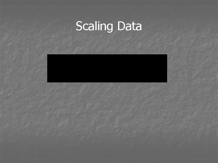
Preparing Data Scaling and normalization: • Scaling - Applying a scale factor and a offset to each raw value; do it same for training, test, and validation sets • Normalization - Sets the n-dimensional input vector to a total Euclidean length of 1 • Z-axis normalization - Retains information on parameter absolute magnitudes lost in normalization

Scaling Data

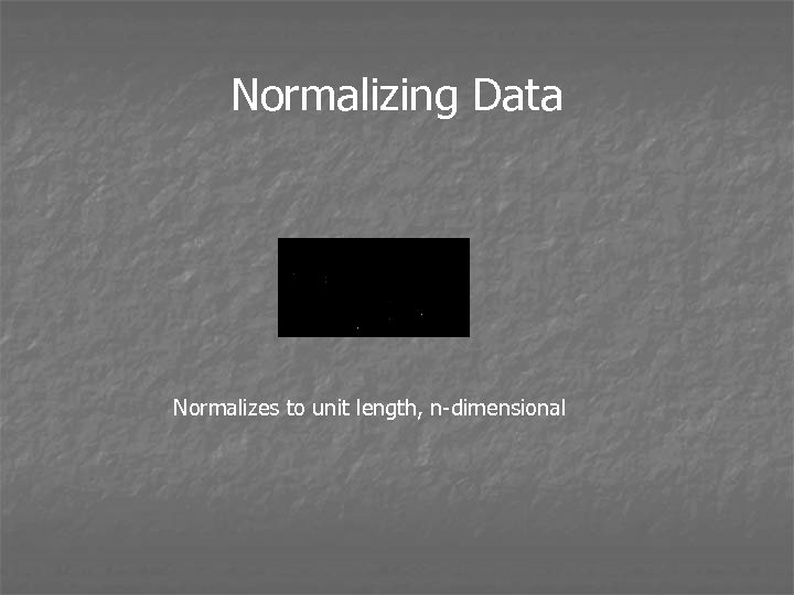Normalizing Data Normalizes to unit length, n-dimensional

Z-axis Normalization 1. Scale each parameter; [-1, 1] for example (now maximum Euclidean length for entire vector is sqrt(n)) 2. Create another input dimension by creating a synthetic variable s for each pattern 3. Calculate z-axis normalized pattern elements; now have n+1 inputs per pattern Note: Not good if most values are near 0, s near 1 is then the dominant parameter in the input

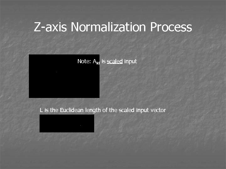Z-axis Normalization Process Note: Aki is scaled input L is the Euclidean length of the scaled input vector

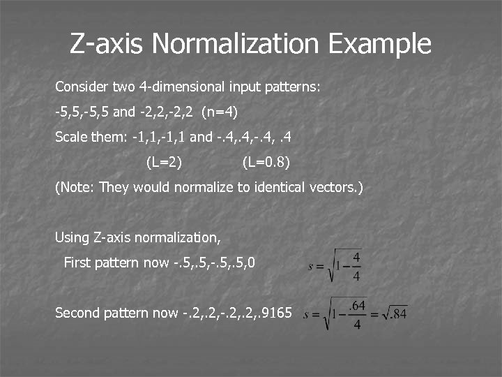Z-axis Normalization Example Consider two 4 -dimensional input patterns: -5, 5, -5, 5 and -2, 2, -2, 2 (n=4) Scale them: -1, 1, -1, 1 and -. 4, . 4 (L=2) (L=0. 8) (Note: They would normalize to identical vectors. ) Using Z-axis normalization, First pattern now -. 5, 0 Second pattern now -. 2, . 9165

Pattern Presentation, and Adding Noise • Order of pattern presentation should be considered during training • Order usually cannot be controlled in final use • May be good to randomize training patterns, especially for online training (can also “shuffle” patterns after each epoch) • Adding noise can result in smoothing of target, and can be useful when limited quantity of training data available

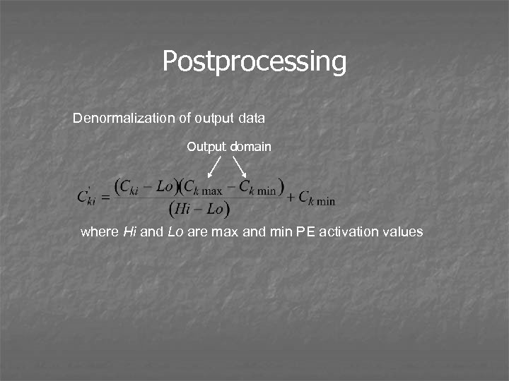Postprocessing Denormalization of output data Output domain where Hi and Lo are max and min PE activation values