Chapter 5 Image Restoration What is Image

Chapter 5 Image Restoration

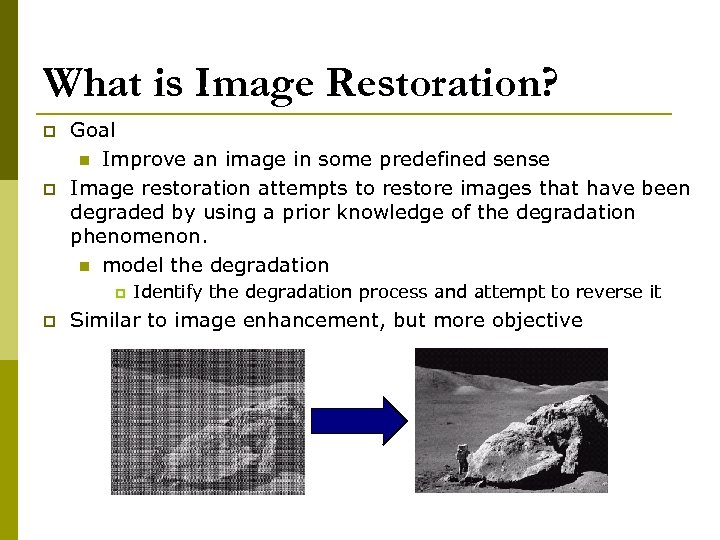What is Image Restoration? p p Goal n Improve an image in some predefined sense Image restoration attempts to restore images that have been degraded by using a prior knowledge of the degradation phenomenon. n model the degradation p p Identify the degradation process and attempt to reverse it Similar to image enhancement, but more objective

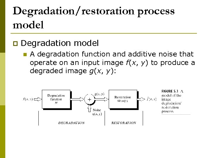Degradation/restoration process model p Degradation model n A degradation function and additive noise that operate on an input image f(x, y) to produce a degraded image g(x, y):

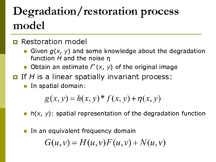Degradation/restoration process model p Restoration model n n p Given g(x, y) and some knowledge about the degradation function H and the noise η Obtain an estimate fˆ(x, y) of the original image If H is a linear spatially invariant process: n In spatial domain: n h(x, y): spatial representation of the degradation function n In an equivalent frequency domain

Sources of noise p Arise during image acquisition (digitization) and/or transmission n p Environmental conditions: light, temperature, humidity, atmospheric disturbance. . . Quality of sensing elements and transmission media Human interference (Transmition) Assumptions of noise (except spatially periodic noise) n n Independent of spatial coordinates Uncorrelated with respect to the image itself

Noise Model p Spatial noise n p Noise models n p Considered as random variables, characterized by a probability density function (PDF) Simulate the behavior and effect of noise There are many different models for the image noise term η(x, y) n Gaussian p n n n Most common model Rayleigh Erlang Exponential Uniform Impulse p Salt and pepper noise

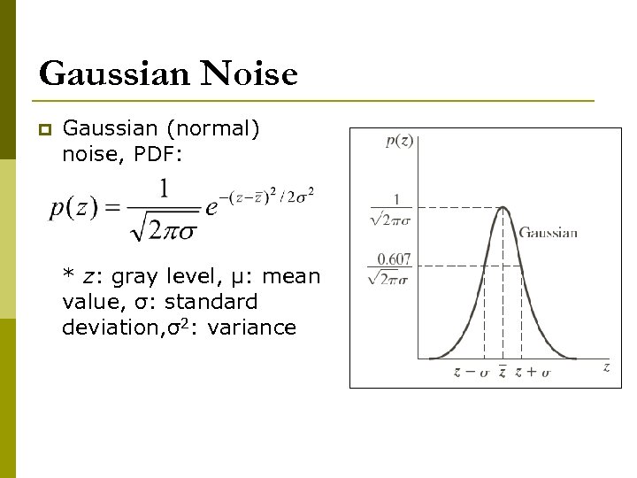Gaussian Noise p Gaussian (normal) noise, PDF: * z: gray level, μ: mean value, σ: standard deviation, σ2: variance

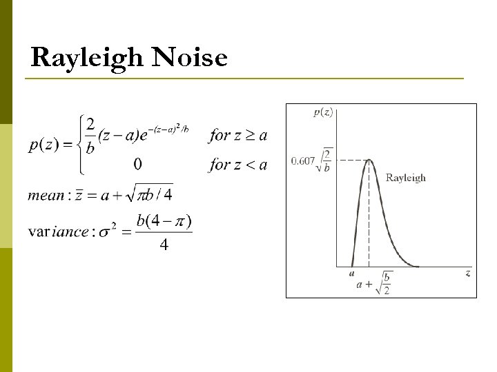Rayleigh Noise

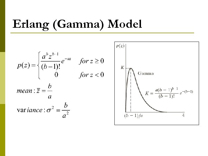Erlang (Gamma) Model

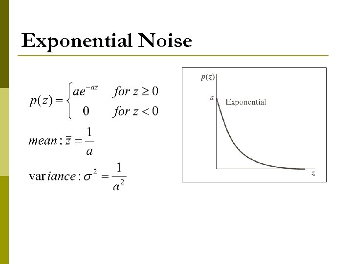Exponential Noise

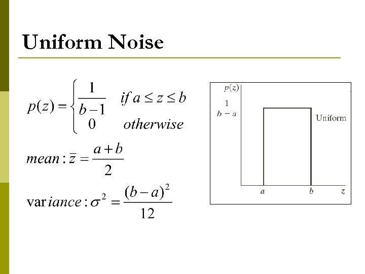Uniform Noise

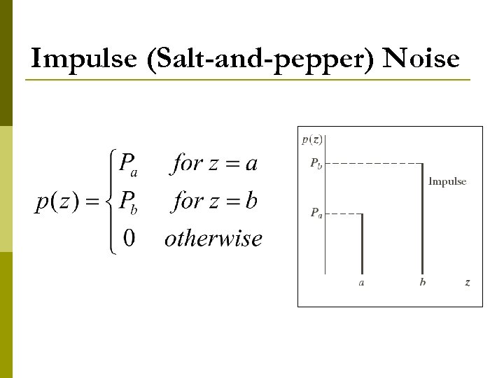Impulse (Salt-and-pepper) Noise

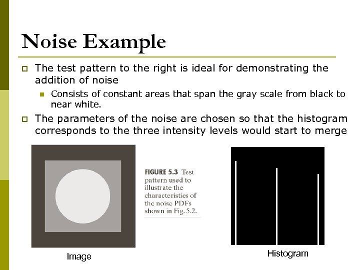Noise Example p The test pattern to the right is ideal for demonstrating the addition of noise n p Consists of constant areas that span the gray scale from black to near white. The parameters of the noise are chosen so that the histogram corresponds to the three intensity levels would start to merge Histogram to go here Image Histogram

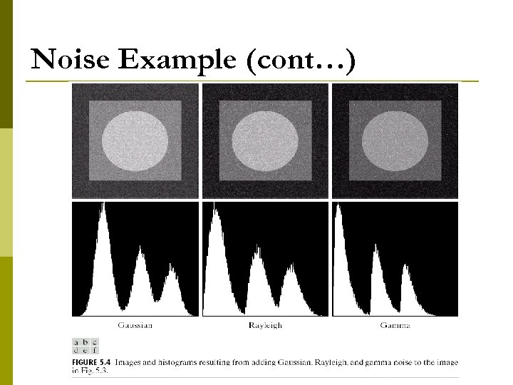Noise Example (cont…)

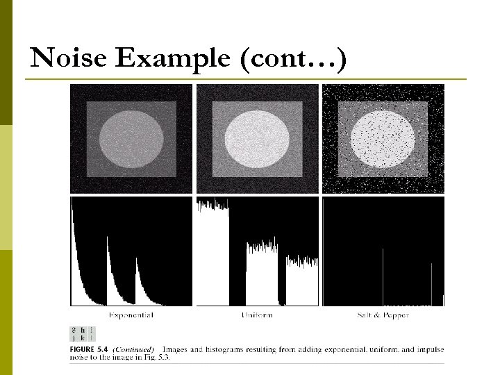Noise Example (cont…)

Periodic Noise Typically arises from electrical or electromechanical interference during image acquisition. p Spatial dependent noise p FT of a pure sinusoid is a pair of conjugate impulses located at the conjugate frequencies of sine wave. p More in section 5. 4 p

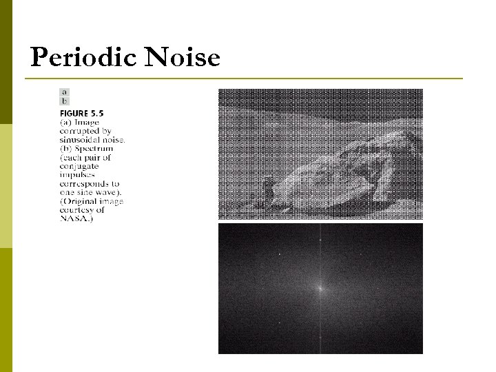Periodic Noise

Estimation of Noise Parameters p Periodic noise parameters typically are estimated by inspection of the FT. n p p Periodic noise tends to produce frequency spikes. Try to infer the periodicity of noise components directly from the image (simple case only) Automated analysis is possible when knowledge is available about the general location of the frequency components

Estimation of Noise Parameters The parameters of noise PDFs may be known partially from sensor specifications p But its necessary to estimate them form images. p n n n Capture a set of images of flat environment. In the case of optical sensors, this is simple as imaging a solid board that is illuminated uniformly. The resulting images are good indicators of system noise.

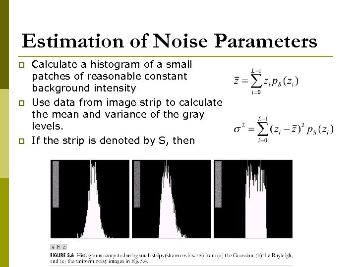Estimation of Noise Parameters p p p Calculate a histogram of a small patches of reasonable constant background intensity Use data from image strip to calculate the mean and variance of the gray levels. If the strip is denoted by S, then

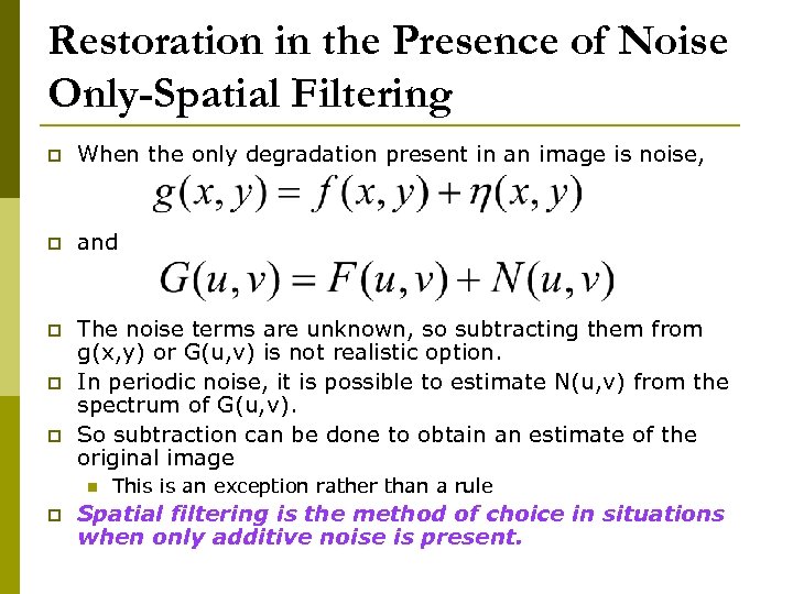Restoration in the Presence of Noise Only-Spatial Filtering p When the only degradation present in an image is noise, p and p The noise terms are unknown, so subtracting them from g(x, y) or G(u, v) is not realistic option. In periodic noise, it is possible to estimate N(u, v) from the spectrum of G(u, v). So subtraction can be done to obtain an estimate of the original image p p n p This is an exception rather than a rule Spatial filtering is the method of choice in situations when only additive noise is present.

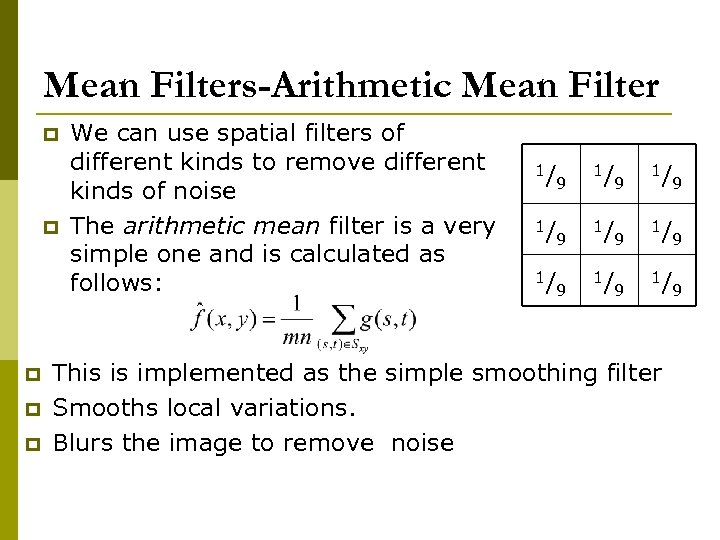Mean Filters-Arithmetic Mean Filter p p p We can use spatial filters of different kinds to remove different kinds of noise The arithmetic mean filter is a very simple one and is calculated as follows: 1/ 9 1/ 9 1/ 9 This is implemented as the simple smoothing filter Smooths local variations. Blurs the image to remove noise

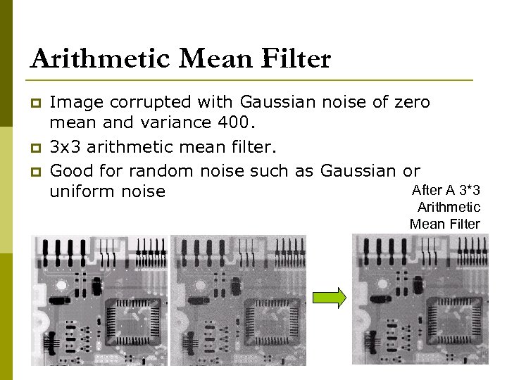Arithmetic Mean Filter p p p Image corrupted with Gaussian noise of zero mean and variance 400. 3 x 3 arithmetic mean filter. Good for random noise such as Gaussian or After A 3*3 uniform noise Arithmetic Mean Filter

Other Means p There are different kinds of mean filters all of which exhibit slightly different behaviour: n n n Geometric Mean Harmonic Mean Contraharmonic Mean

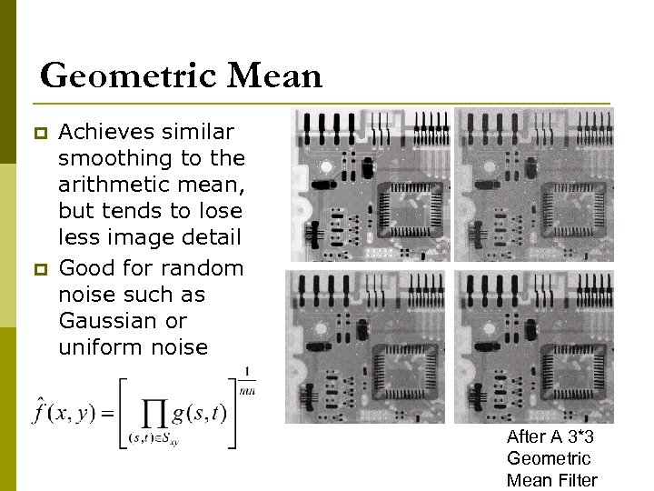Geometric Mean p p Achieves similar smoothing to the arithmetic mean, but tends to lose less image detail Good for random noise such as Gaussian or uniform noise After A 3*3 Geometric Mean Filter

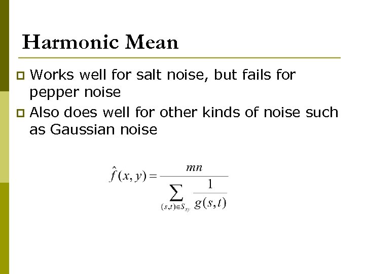Harmonic Mean Works well for salt noise, but fails for pepper noise p Also does well for other kinds of noise such as Gaussian noise p

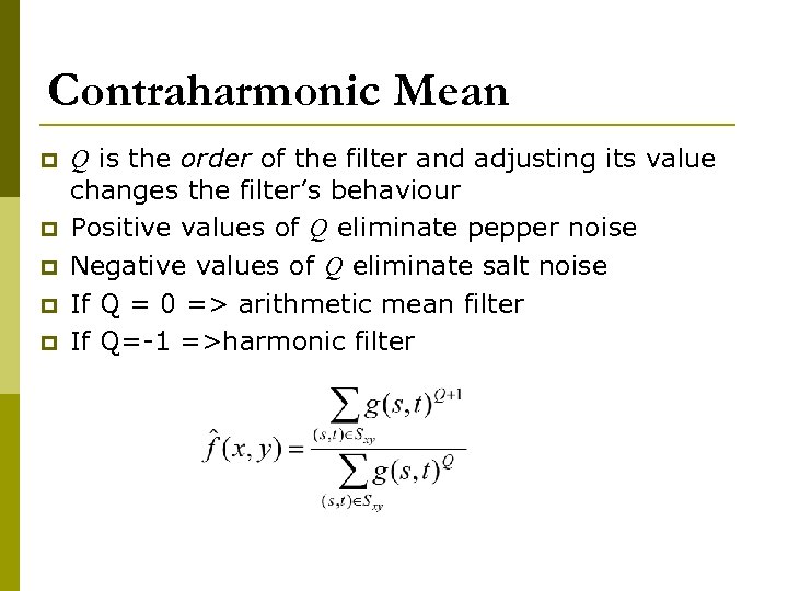Contraharmonic Mean p p p Q is the order of the filter and adjusting its value changes the filter’s behaviour Positive values of Q eliminate pepper noise Negative values of Q eliminate salt noise If Q = 0 => arithmetic mean filter If Q=-1 =>harmonic filter

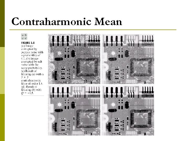Contraharmonic Mean

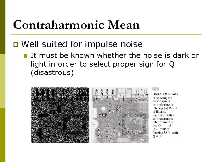Contraharmonic Mean p Well suited for impulse noise n It must be known whether the noise is dark or light in order to select proper sign for Q (disastrous)

Order Statistics Filters Spatial filters that are based on ordering the pixel values that make up the neighbourhood operated on by the filter p Useful spatial filters include p n n Median filter Max and min filter Midpoint filter Alpha trimmed mean filter

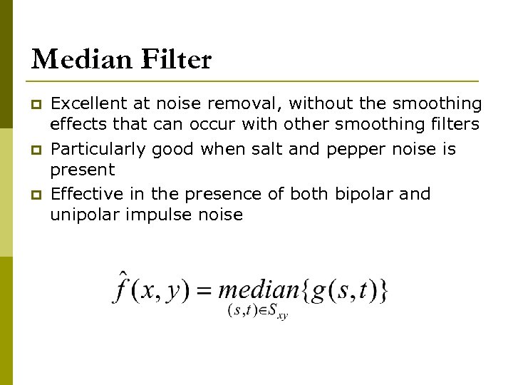Median Filter p p p Excellent at noise removal, without the smoothing effects that can occur with other smoothing filters Particularly good when salt and pepper noise is present Effective in the presence of both bipolar and unipolar impulse noise

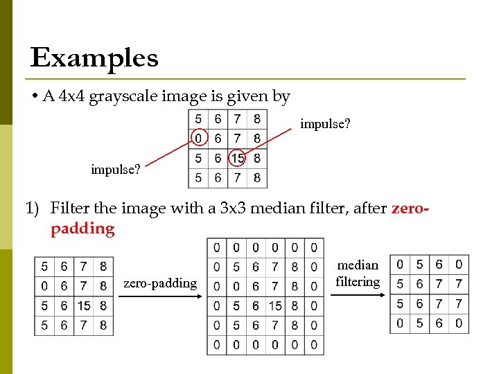Examples • A 4 x 4 grayscale image is given by impulse? 1) Filter the image with a 3 x 3 median filter, after zeropadding at the image borders zero-padding median filtering

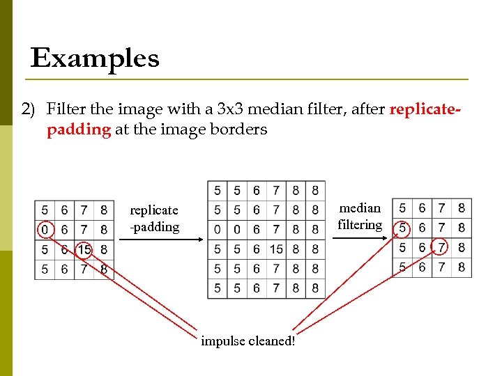Examples 2) Filter the image with a 3 x 3 median filter, after replicatepadding at the image borders median filtering replicate -padding impulse cleaned!

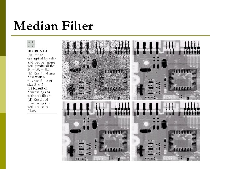Median Filter

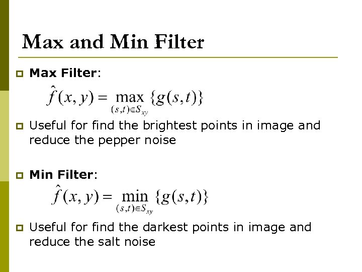Max and Min Filter p Max Filter: p Useful for find the brightest points in image and reduce the pepper noise p Min Filter: p Useful for find the darkest points in image and reduce the salt noise

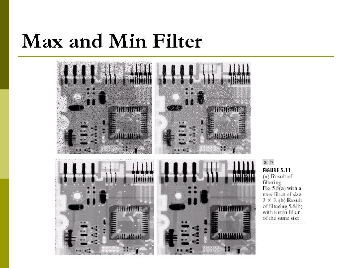Max and Min Filter

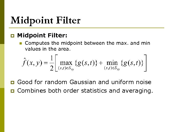Midpoint Filter p Midpoint Filter: n p p Computes the midpoint between the max. and min values in the area. Good for random Gaussian and uniform noise Combines both order statistics and averaging.

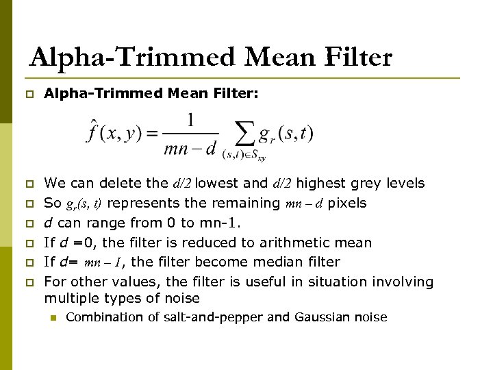Alpha-Trimmed Mean Filter p Alpha-Trimmed Mean Filter: p We can delete the d/2 lowest and d/2 highest grey levels So gr(s, t) represents the remaining mn – d pixels d can range from 0 to mn-1. If d =0, the filter is reduced to arithmetic mean If d= mn – 1, the filter become median filter For other values, the filter is useful in situation involving multiple types of noise p p p n Combination of salt-and-pepper and Gaussian noise

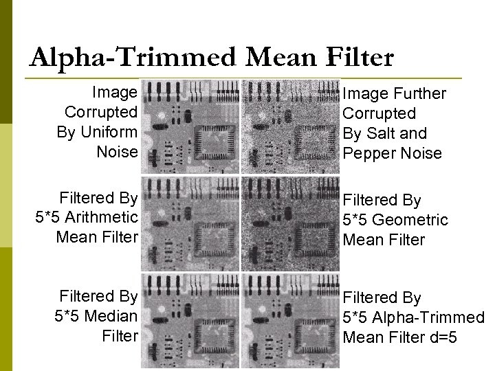Alpha-Trimmed Mean Filter Image Corrupted By Uniform Noise Image Further Corrupted By Salt and Pepper Noise Filtered By 5*5 Arithmetic Mean Filtered By 5*5 Geometric Mean Filtered By 5*5 Median Filtered By 5*5 Alpha-Trimmed Mean Filter d=5

Adaptive Filters The filters discussed so far are applied to an entire image without any regard for how image characteristics vary from one point to another p The behaviour of adaptive filters changes depending on the characteristics of the image inside the filter region p Superior performance compared to filters discussed so far p We will take a look at the adaptive median filter p

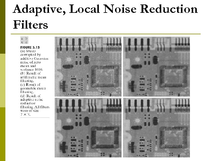
Adaptive, Local Noise Reduction Filters p p Statistical measures of a random variables are closely related to appearance of an image Adaptive filter is based on these quantities (mean, variance) n n p Mean gives a measure of average intensity Variance gives a measure of contrast The filter response at any point (x, y) is based on four quantities: n n g(x, y): the value of the noisy image at (x, y) The variance of the noise corrupting f(x, y) to form g(x, y) The local mean of the pixels in Sxy The local variance of the pixels in Sxy

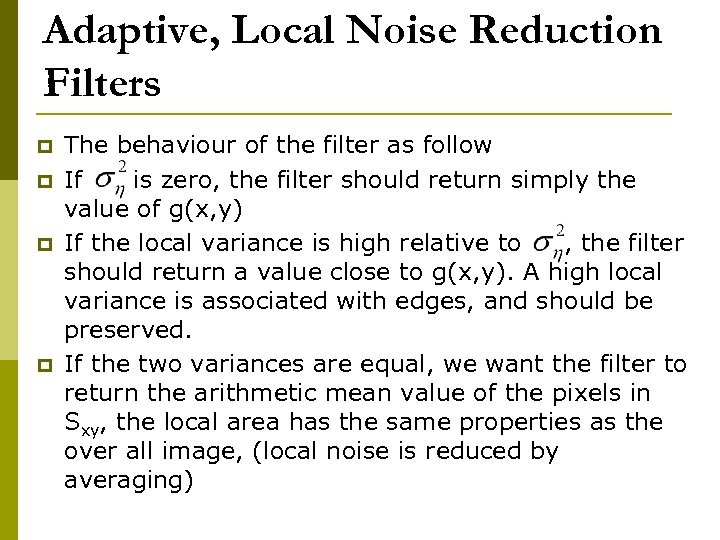Adaptive, Local Noise Reduction Filters p p The behaviour of the filter as follow If is zero, the filter should return simply the value of g(x, y) If the local variance is high relative to , the filter should return a value close to g(x, y). A high local variance is associated with edges, and should be preserved. If the two variances are equal, we want the filter to return the arithmetic mean value of the pixels in Sxy, the local area has the same properties as the over all image, (local noise is reduced by averaging)

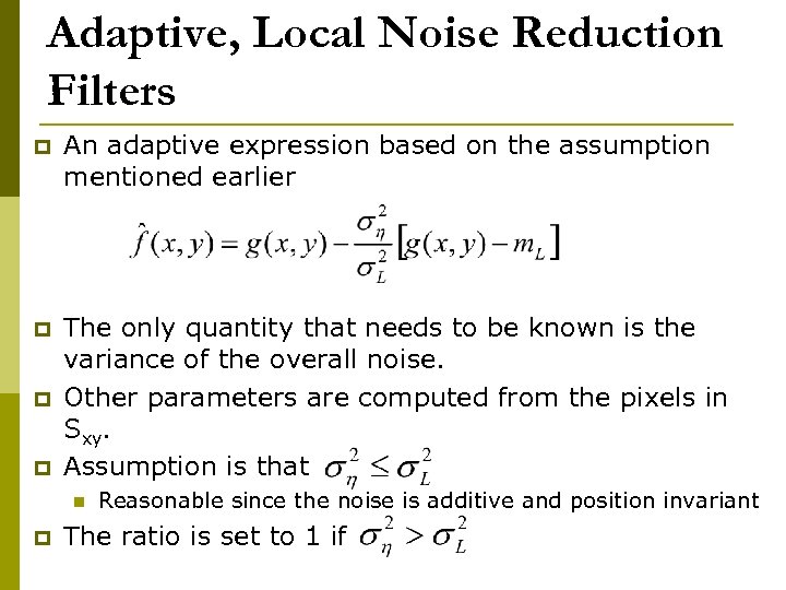Adaptive, Local Noise Reduction Filters p An adaptive expression based on the assumption mentioned earlier p The only quantity that needs to be known is the variance of the overall noise. Other parameters are computed from the pixels in Sxy. Assumption is that p p n p Reasonable since the noise is additive and position invariant The ratio is set to 1 if

Adaptive, Local Noise Reduction Filters

Adaptive Median Filtering The median filter performs relatively well on impulse noise as long as the spatial density of the impulse noise is not large (Pa and Pb less than 0. 2) p The adaptive median filter can handle much more spatially dense impulse noise, and also performs some smoothing for nonimpulse noise p The key insight in the adaptive median filter is that the filter size changes depending on the characteristics of the image p

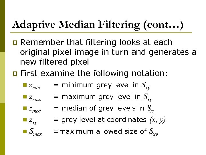Adaptive Median Filtering (cont…) Remember that filtering looks at each original pixel image in turn and generates a new filtered pixel p First examine the following notation: n zmin = minimum grey level in Sxy n zmax = maximum grey level in Sxy n zmed = median of grey levels in Sxy n zxy = grey level at coordinates (x, y) n Smax =maximum allowed size of Sxy p

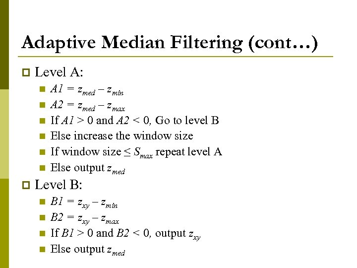Adaptive Median Filtering (cont…) p Level A: n n n p A 1 = zmed – zmin A 2 = zmed – zmax If A 1 > 0 and A 2 < 0, Go to level B Else increase the window size If window size ≤ Smax repeat level A Else output zmed Level B: n n B 1 = zxy – zmin B 2 = zxy – zmax If B 1 > 0 and B 2 < 0, output zxy Else output zmed

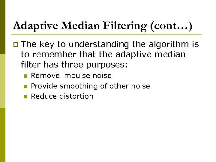Adaptive Median Filtering (cont…) p The key to understanding the algorithm is to remember that the adaptive median filter has three purposes: n n n Remove impulse noise Provide smoothing of other noise Reduce distortion

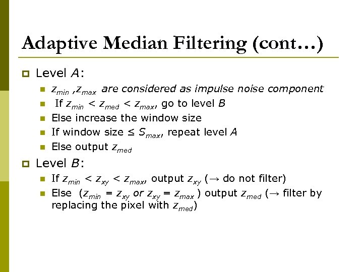Adaptive Median Filtering (cont…) p Level A: n n n p zmin , zmax are considered as impulse noise component If zmin < zmed < zmax, go to level B Else increase the window size If window size ≤ Smax, repeat level A Else output zmed Level B: n n If zmin < zxy < zmax, output zxy (→ do not filter) Else (zmin = zxy or zxy = zmax ) output zmed (→ filter by replacing the pixel with zmed)

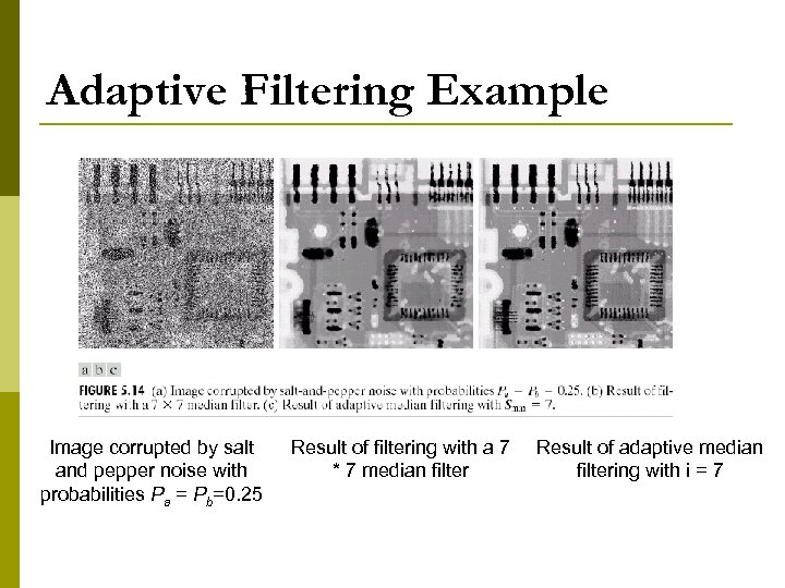Adaptive Filtering Example Image corrupted by salt and pepper noise with probabilities Pa = Pb=0. 25 Result of filtering with a 7 * 7 median filter Result of adaptive median filtering with i = 7

Periodic Noise p Gives rise to regular noise patterns in an image p Frequency domain techniques in the Fourier domain are most effective at removing periodic noise

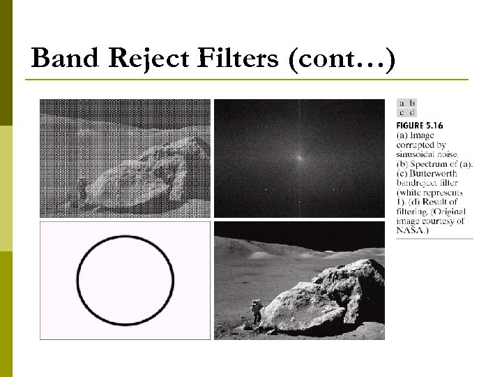
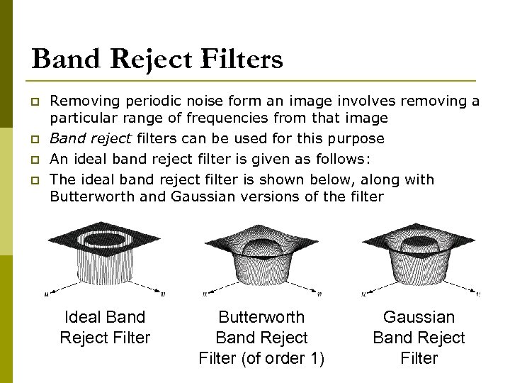Band Reject Filters p p Removing periodic noise form an image involves removing a particular range of frequencies from that image Band reject filters can be used for this purpose An ideal band reject filter is given as follows: The ideal band reject filter is shown below, along with Butterworth and Gaussian versions of the filter Ideal Band Reject Filter Butterworth Band Reject Filter (of order 1) Gaussian Band Reject Filter

Band Reject Filters (cont…)

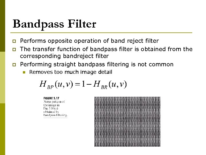Bandpass Filter p p p Performs opposite operation of band reject filter The transfer function of bandpass filter is obtained from the corresponding bandreject filter Performing straight bandpass filtering is not common n Removes too much image detail

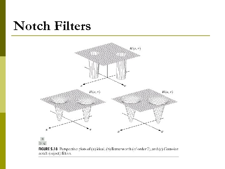Notch Filters

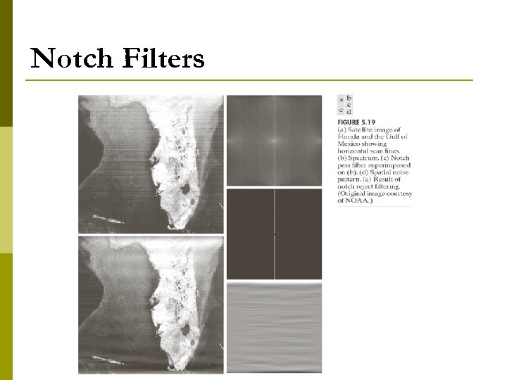Notch Filters

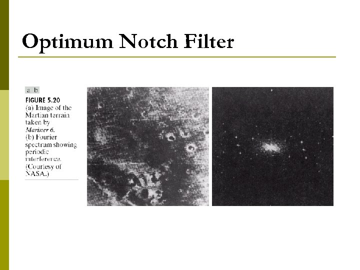Optimum Notch Filter

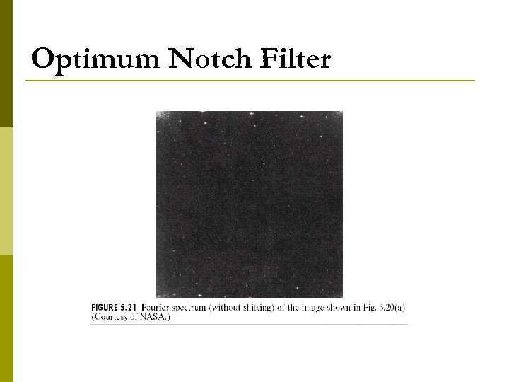
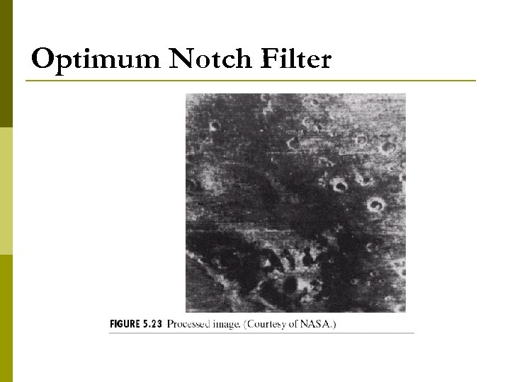
Optimum Notch Filter p When several interference components are present, the normal methods are not always acceptable n Remove too much image information. The interference components generally are not single frequency bursts. p Optimum in the sense that it minimizes the local variance of the restored image. p

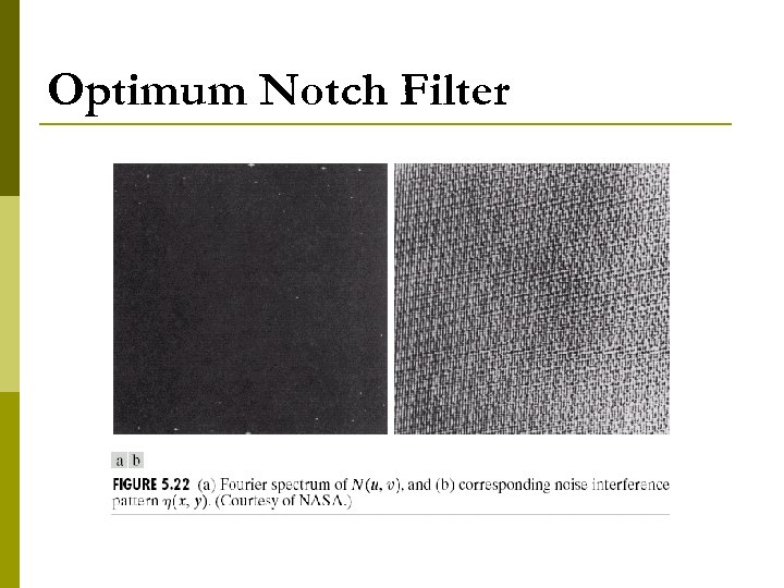
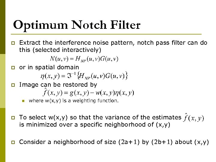Optimum Notch Filter p Extract the interference noise pattern, notch pass filter can do this (selected interactively) p or in spatial domain p Image can be restored by n where w(x, y) is a weighting function. p To select w(x, y) so that the variance of the estimates is minimized over a specific neighborhood of (x, y) p Consider a neighborhood of size (2 a+1) by (2 b+1) about (x, y)

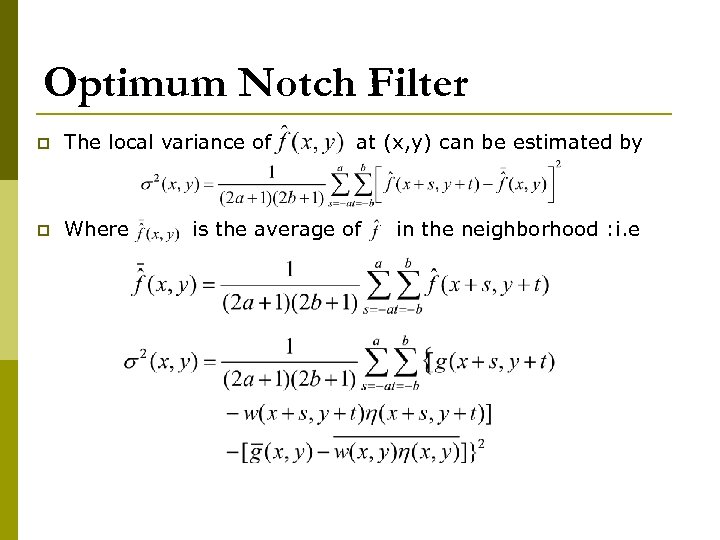Optimum Notch Filter p The local variance of p Where at (x, y) can be estimated by is the average of in the neighborhood : i. e

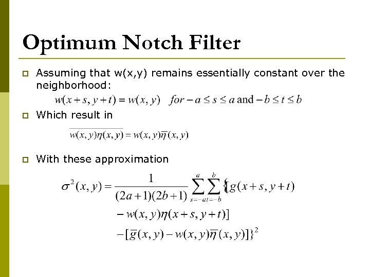Optimum Notch Filter p Assuming that w(x, y) remains essentially constant over the neighborhood: p Which result in p With these approximation

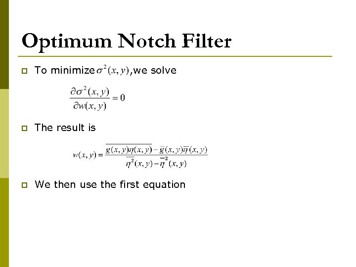Optimum Notch Filter p To minimize , we solve p The result is p We then use the first equation

Optimum Notch Filter

Optimum Notch Filter

Optimum Notch Filter

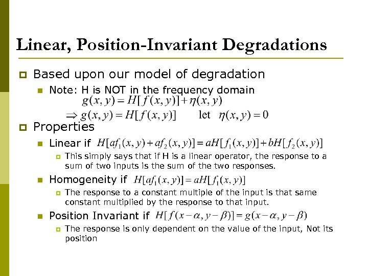Linear, Position-Invariant Degradations p Based upon our model of degradation n p Note: H is NOT in the frequency domain Properties n Linear if p n Homogeneity if p n This simply says that if H is a linear operator, the response to a sum of two inputs is the sum of the two responses. The response to a constant multiple of the input is that same constant multiplied by the response to that input. Position Invariant if p The response is only dependent on the value of the input, Not its position

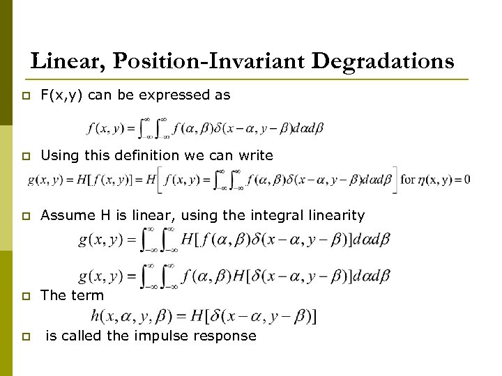Linear, Position-Invariant Degradations p F(x, y) can be expressed as p Using this definition we can write p Assume H is linear, using the integral linearity p The term p is called the impulse response

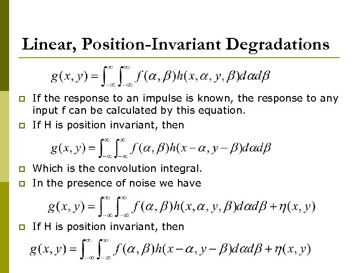Linear, Position-Invariant Degradations p p If the response to an impulse is known, the response to any input f can be calculated by this equation. If H is position invariant, then p Which is the convolution integral. In the presence of noise we have p If H is position invariant, then p

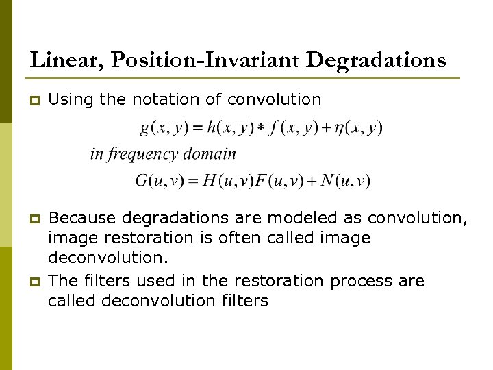Linear, Position-Invariant Degradations p Using the notation of convolution p Because degradations are modeled as convolution, image restoration is often called image deconvolution. The filters used in the restoration process are called deconvolution filters p

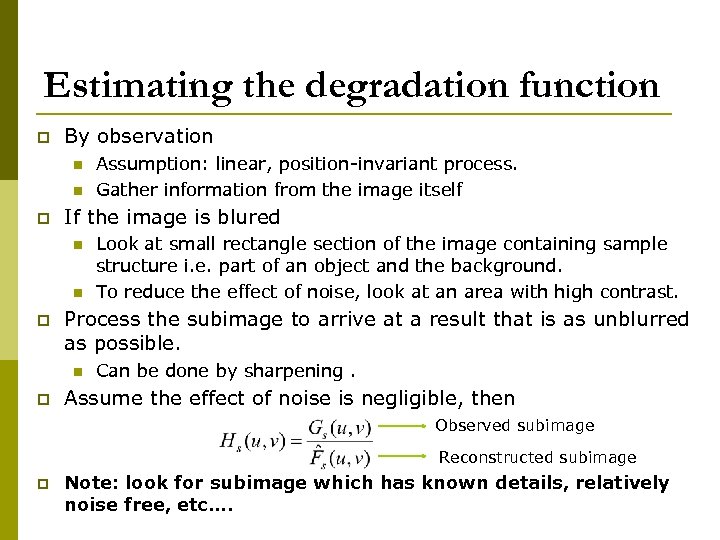Estimating the degradation function p By observation n n p If the image is blured n n p Look at small rectangle section of the image containing sample structure i. e. part of an object and the background. To reduce the effect of noise, look at an area with high contrast. Process the subimage to arrive at a result that is as unblurred as possible. n p Assumption: linear, position-invariant process. Gather information from the image itself Can be done by sharpening. Assume the effect of noise is negligible, then Observed subimage Reconstructed subimage p Note: look for subimage which has known details, relatively noise free, etc….

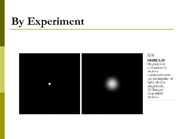
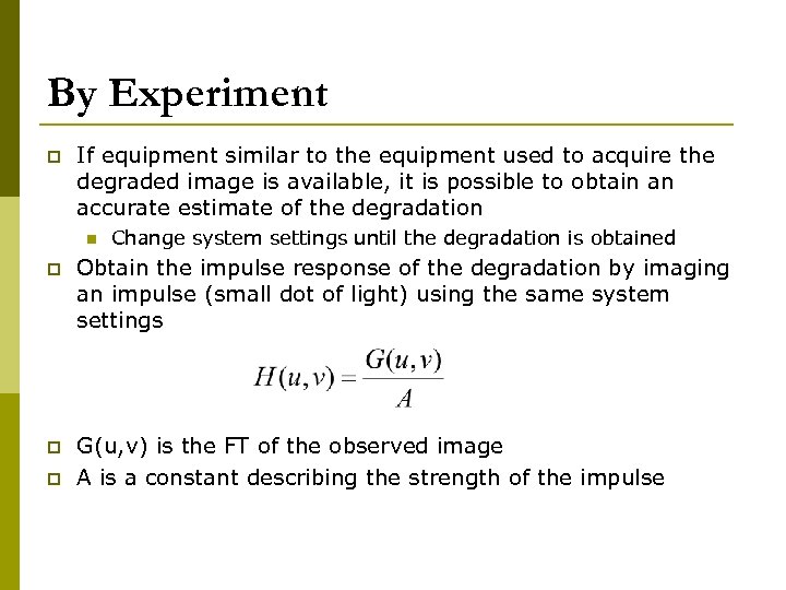By Experiment p If equipment similar to the equipment used to acquire the degraded image is available, it is possible to obtain an accurate estimate of the degradation n Change system settings until the degradation is obtained p Obtain the impulse response of the degradation by imaging an impulse (small dot of light) using the same system settings p G(u, v) is the FT of the observed image A is a constant describing the strength of the impulse p

By Experiment

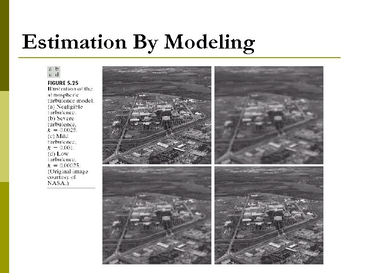
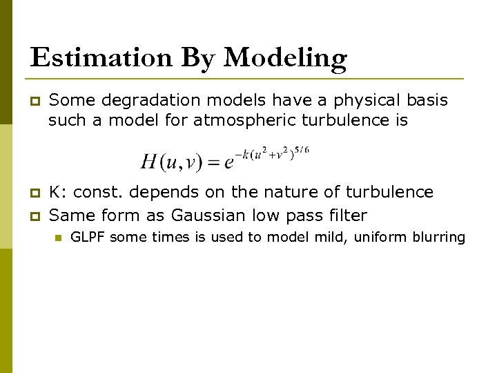Estimation By Modeling p Some degradation models have a physical basis such a model for atmospheric turbulence is p K: const. depends on the nature of turbulence Same form as Gaussian low pass filter p n GLPF some times is used to model mild, uniform blurring

Estimation By Modeling

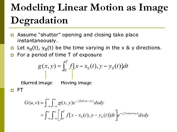Modeling Linear Motion as Image Degradation p p p Assume “shutter” opening and closing take place instantaneously. Let x 0(t), y 0(t) be the time varying in the x & y directions. For a period of time T of exposure Blurred image p FT Moving image

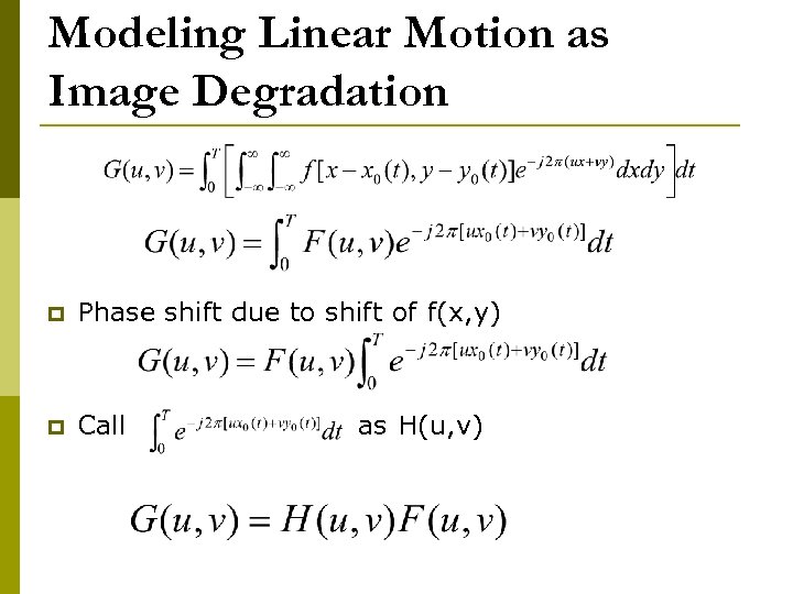Modeling Linear Motion as Image Degradation p Phase shift due to shift of f(x, y) p Call as H(u, v)

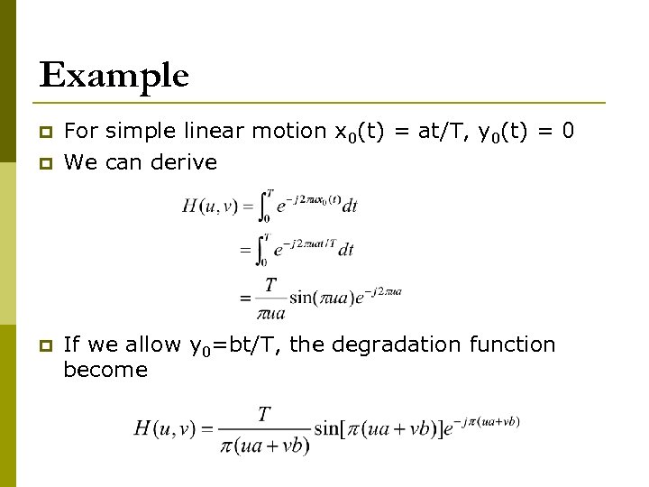Example p p p For simple linear motion x 0(t) = at/T, y 0(t) = 0 We can derive If we allow y 0=bt/T, the degradation function become

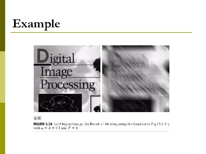Example

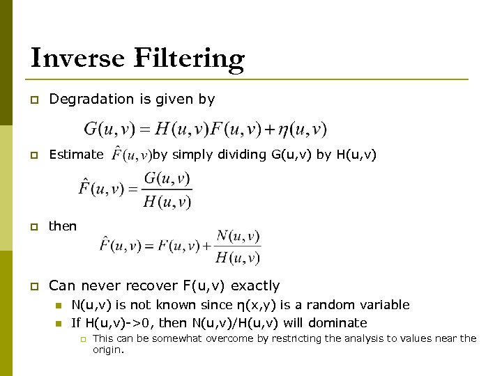Inverse Filtering p Degradation is given by p Estimate p then p Can never recover F(u, v) exactly n n by simply dividing G(u, v) by H(u, v) N(u, v) is not known since η(x, y) is a random variable If H(u, v)->0, then N(u, v)/H(u, v) will dominate p This can be somewhat overcome by restricting the analysis to values near the origin.

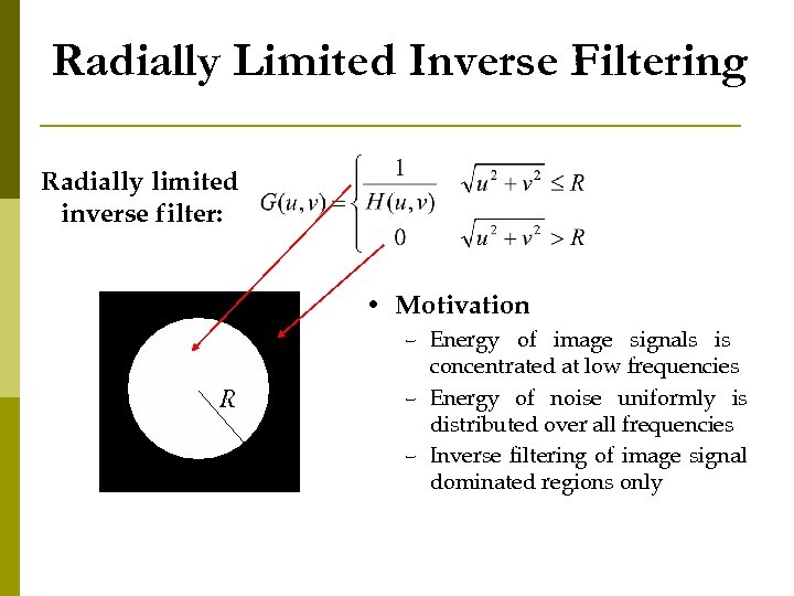Radially Limited Inverse Filtering Radially limited inverse filter: • Motivation R – Energy of image signals is concentrated at low frequencies – Energy of noise uniformly is distributed over all frequencies – Inverse filtering of image signal dominated regions only

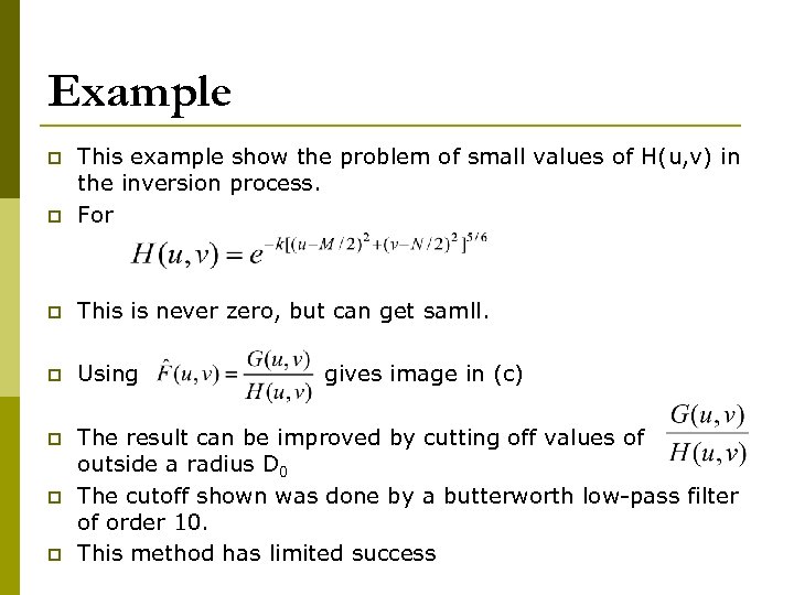Example p This example show the problem of small values of H(u, v) in the inversion process. For p This is never zero, but can get samll. p Using p The result can be improved by cutting off values of outside a radius D 0 The cutoff shown was done by a butterworth low-pass filter of order 10. This method has limited success p p p gives image in (c)

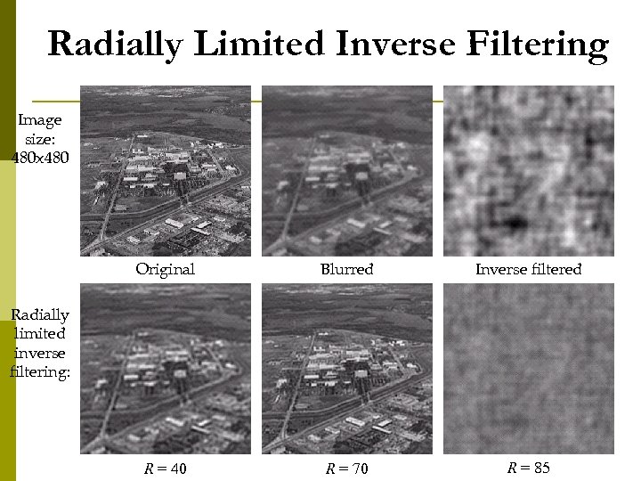Radially Limited Inverse Filtering Image size: 480 x 480 Original Blurred Inverse filtered R = 40 R = 70 R = 85 Radially limited inverse filtering:

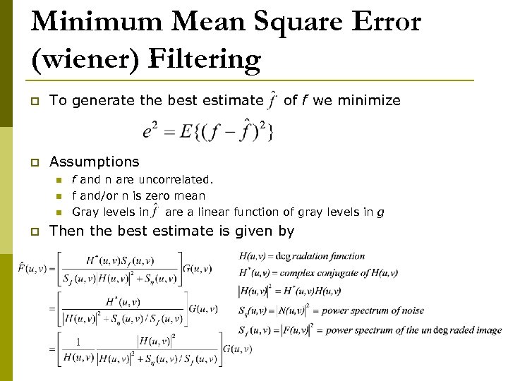Minimum Mean Square Error (wiener) Filtering p To generate the best estimate p Assumptions n n n p of f we minimize f and n are uncorrelated. f and/or n is zero mean Gray levels in are a linear function of gray levels in g Then the best estimate is given by

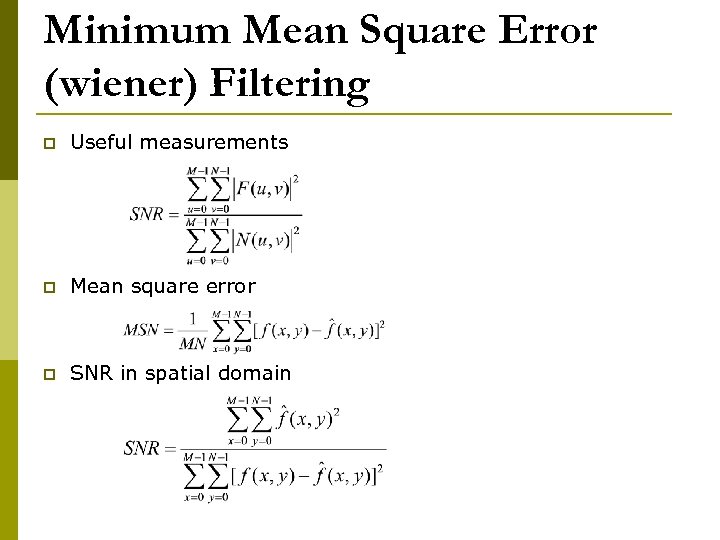Minimum Mean Square Error (wiener) Filtering p Useful measurements p Mean square error p SNR in spatial domain

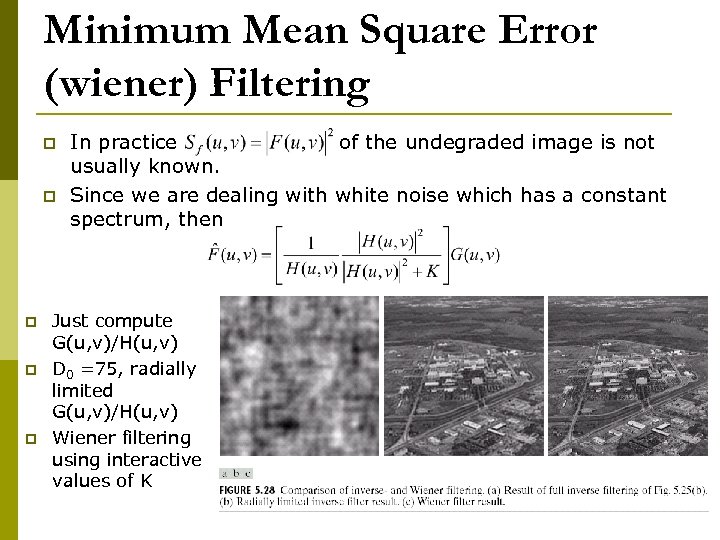Minimum Mean Square Error (wiener) Filtering p p p In practice of the undegraded image is not usually known. Since we are dealing with white noise which has a constant spectrum, then Just compute G(u, v)/H(u, v) D 0 =75, radially limited G(u, v)/H(u, v) Wiener filtering using interactive values of K

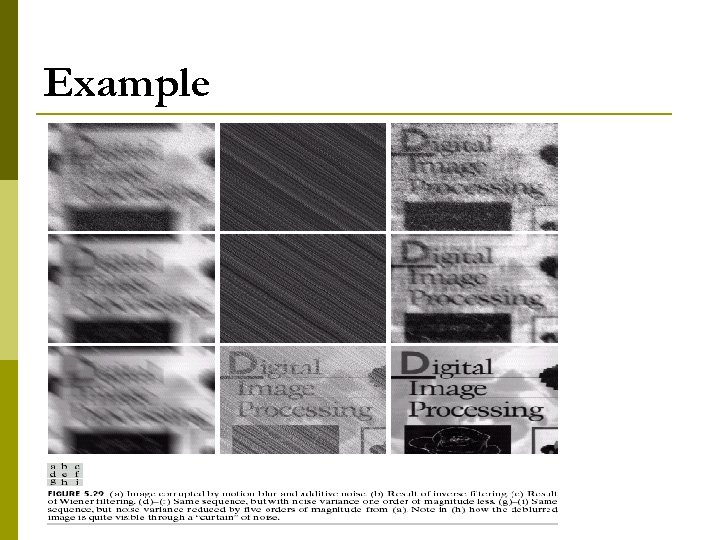Example

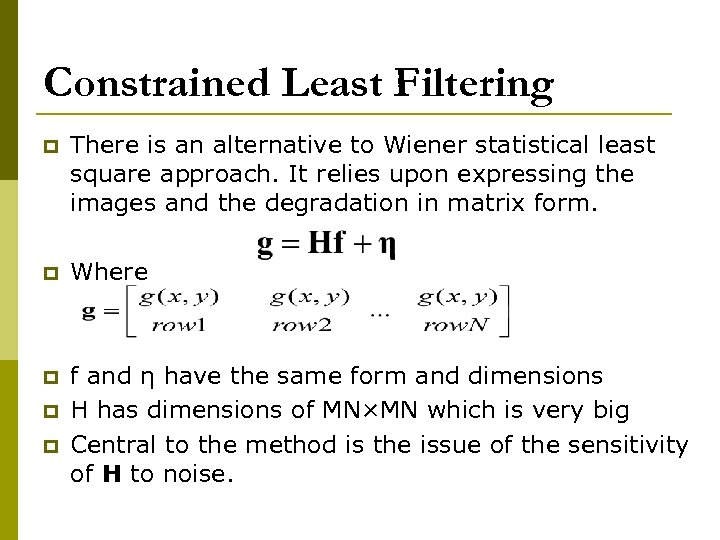Constrained Least Filtering p There is an alternative to Wiener statistical least square approach. It relies upon expressing the images and the degradation in matrix form. p Where p f and η have the same form and dimensions H has dimensions of MN×MN which is very big Central to the method is the issue of the sensitivity of H to noise. p p

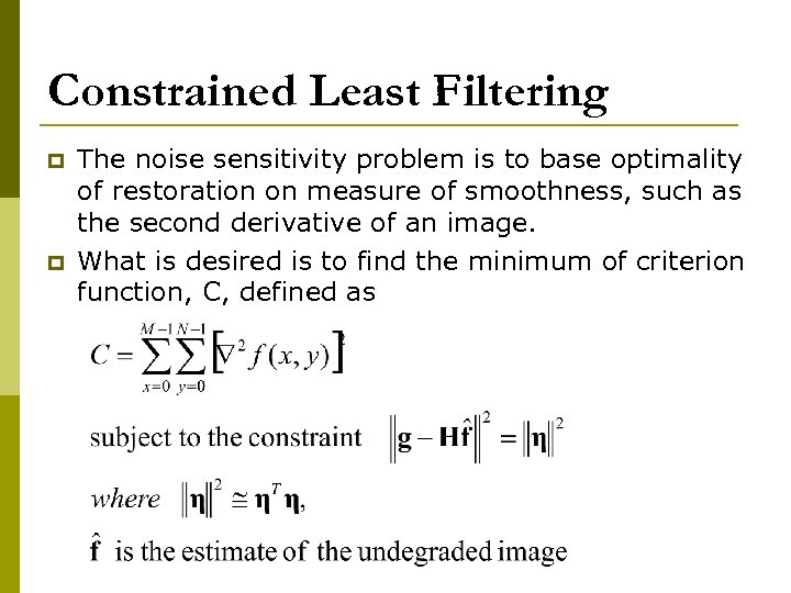Constrained Least Filtering p p The noise sensitivity problem is to base optimality of restoration on measure of smoothness, such as the second derivative of an image. What is desired is to find the minimum of criterion function, C, defined as

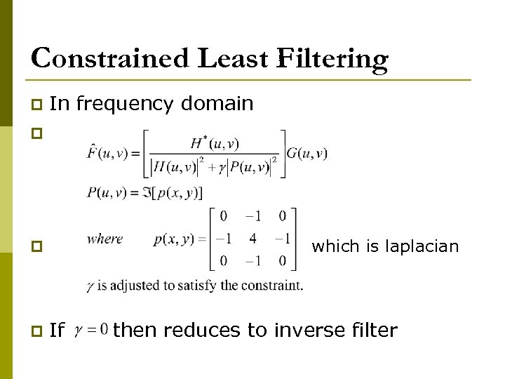Constrained Least Filtering p In frequency domain p which is laplacian p p If then reduces to inverse filter

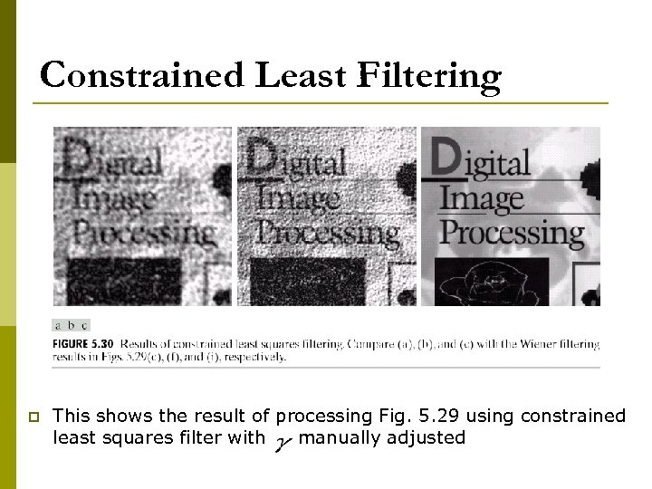Constrained Least Filtering p This shows the result of processing Fig. 5. 29 using constrained least squares filter with manually adjusted

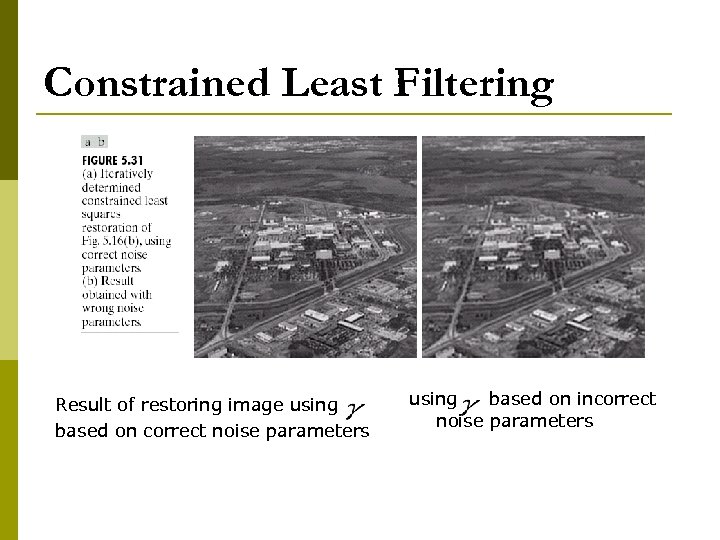Constrained Least Filtering Result of restoring image using based on correct noise parameters using based on incorrect noise parameters