fefa75d0ca0f0685a690f44f6da3ce57.ppt
- Количество слайдов: 22
CHAPTER 5 DISCRETE PROBABILITY DISTRIBUTIONS 1
2
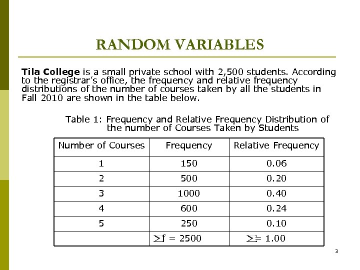
RANDOM VARIABLES Tila College is a small private school with 2, 500 students. According to the registrar’s office, the frequency and relative frequency distributions of the number of courses taken by all the students in Fall 2010 are shown in the table below. Table 1: Frequency and Relative Frequency Distribution of the number of Courses Taken by Students Number of Courses Frequency Relative Frequency 1 150 0. 06 2 500 0. 20 3 1000 0. 40 4 600 0. 24 5 250 0. 10 f = 2500 = 1. 00 3
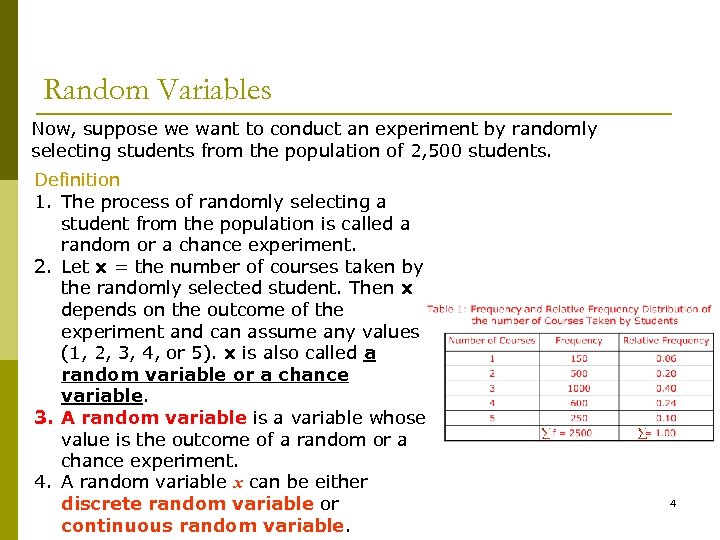
Random Variables Now, suppose we want to conduct an experiment by randomly selecting students from the population of 2, 500 students. Definition 1. The process of randomly selecting a student from the population is called a random or a chance experiment. 2. Let x = the number of courses taken by the randomly selected student. Then x depends on the outcome of the experiment and can assume any values (1, 2, 3, 4, or 5). x is also called a random variable or a chance variable. 3. A random variable is a variable whose value is the outcome of a random or a chance experiment. 4. A random variable x can be either discrete random variable or continuous random variable. 4
Discrete Random Variable Definition p A discrete random variable is a random variable that assumes countable values. p In our example, the number of courses taken by students in Fall 2010 is a discrete random variable because it can assume any value, 1, 2, 3, 4, or 5. p Other examples of discrete random variables are: Ø Ø Ø The number of smokers in STA 12 class The number of cars owned by families in your city The number of fish caught on a fishing trip 5
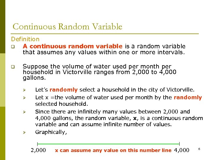
Continuous Random Variable Definition q A continuous random variable is a random variable that assumes any values within one or more intervals. q Suppose the volume of water used per month per household in Victorville ranges from 2, 000 to 4, 000 gallons. Ø Ø Let’s randomly select a household in the city of Victorville. Let x =the volume of water used per month by the randomly selected household. Since there are infinitely many values between 2, 000 and 4, 000 gallons, the random variable, x, is a continuous random variable and can assume infinite number of values. Graphically, 2, 000 x can assume any value on this number line 4, 000 6
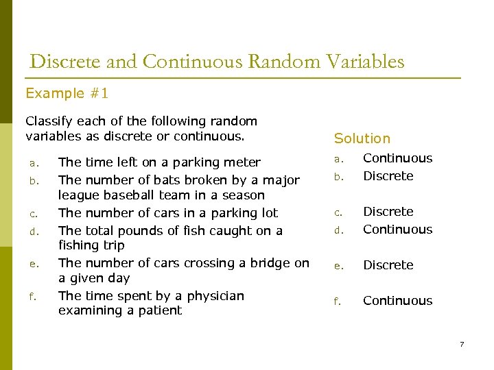
Discrete and Continuous Random Variables Example #1 Classify each of the following random variables as discrete or continuous. a. b. c. d. e. f. The time left on a parking meter The number of bats broken by a major league baseball team in a season The number of cars in a parking lot The total pounds of fish caught on a fishing trip The number of cars crossing a bridge on a given day The time spent by a physician examining a patient Solution a. b. Continuous Discrete d. Discrete Continuous e. Discrete f. Continuous c. 7
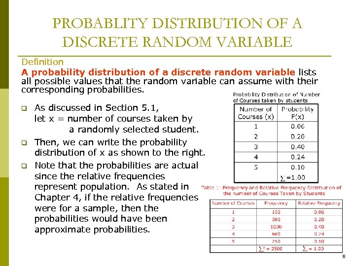
PROBABLITY DISTRIBUTION OF A DISCRETE RANDOM VARIABLE Definition A probability distribution of a discrete random variable lists all possible values that the random variable can assume with their corresponding probabilities. q q q As discussed in Section 5. 1, let x = number of courses taken by a randomly selected student. Then, we can write the probability distribution of x as shown to the right. Note that the probabilities are actual since the relative frequencies represent population. As stated in Chapter 4, if the relative frequencies were for a sample, then the probabilities would have been approximate probabilities. 8
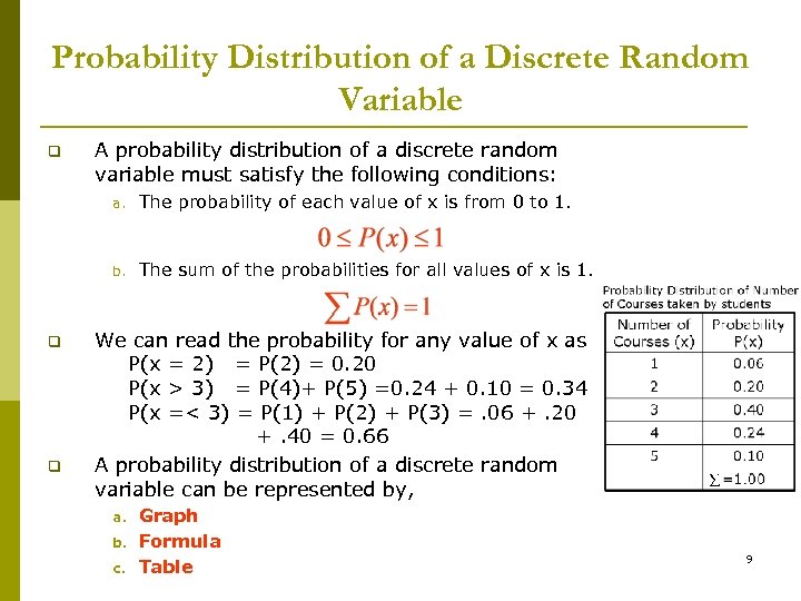
Probability Distribution of a Discrete Random Variable q A probability distribution of a discrete random variable must satisfy the following conditions: a. b. q q The probability of each value of x is from 0 to 1. The sum of the probabilities for all values of x is 1. We can read the probability for any value of x as P(x = 2) = P(2) = 0. 20 P(x > 3) = P(4)+ P(5) =0. 24 + 0. 10 = 0. 34 P(x =< 3) = P(1) + P(2) + P(3) =. 06 +. 20 +. 40 = 0. 66 A probability distribution of a discrete random variable can be represented by, a. b. c. Graph Formula Table 9
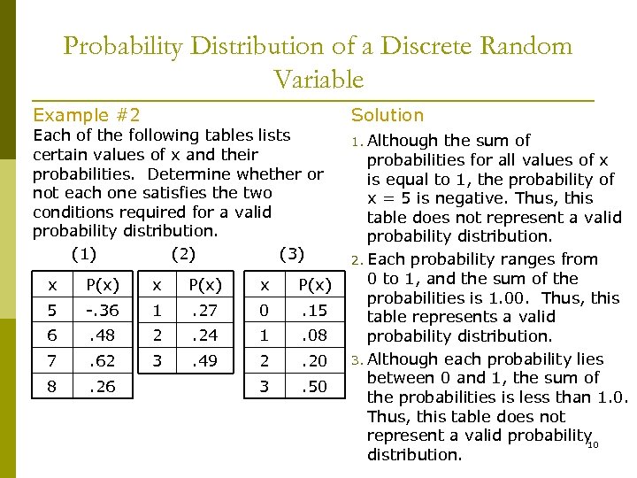
Probability Distribution of a Discrete Random Variable Example #2 Each of the following tables lists certain values of x and their probabilities. Determine whether or not each one satisfies the two conditions required for a valid probability distribution. (1) (2) (3) x P(x) 5 -. 36 1 . 27 0 . 15 6 . 48 2 . 24 1 . 08 7 . 62 3 . 49 2 . 20 8 . 26 3 . 50 Solution 1. Although the sum of probabilities for all values of x is equal to 1, the probability of x = 5 is negative. Thus, this table does not represent a valid probability distribution. 2. Each probability ranges from 0 to 1, and the sum of the probabilities is 1. 00. Thus, this table represents a valid probability distribution. 3. Although each probability lies between 0 and 1, the sum of the probabilities is less than 1. 0. Thus, this table does not represent a valid probability 10 distribution.
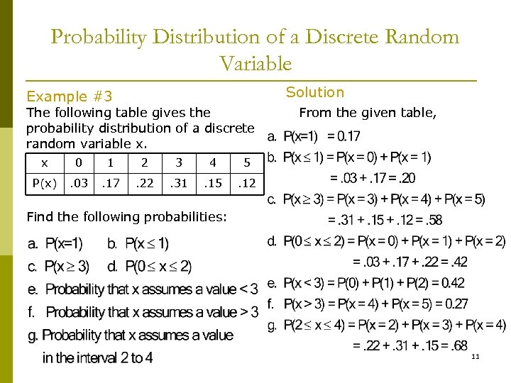
Probability Distribution of a Discrete Random Variable Solution Example #3 The following table gives the probability distribution of a discrete random variable x. x 0 1 2 3 4 5 P(x) . 03 . 17 . 22 . 31 . 15 From the given table, . 12 Find the following probabilities: 11
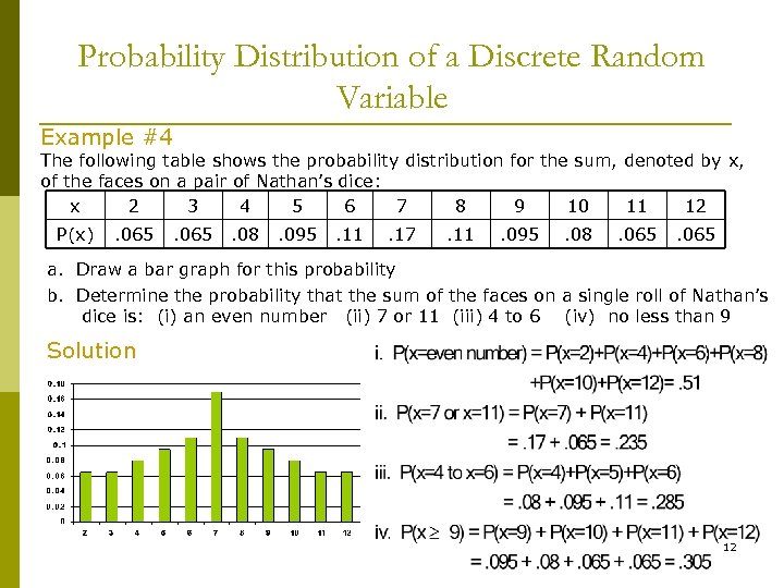
Probability Distribution of a Discrete Random Variable Example #4 The following table shows the probability distribution for the sum, denoted by x, of the faces on a pair of Nathan’s dice: x 2 3 4 5 6 7 8 9 10 11 12 P(x) . 065 . 08 . 095 . 11 . 17 . 11 . 095 . 08 . 065 a. Draw a bar graph for this probability b. Determine the probability that the sum of the faces on a single roll of Nathan’s dice is: (i) an even number (ii) 7 or 11 (iii) 4 to 6 (iv) no less than 9 Solution 12
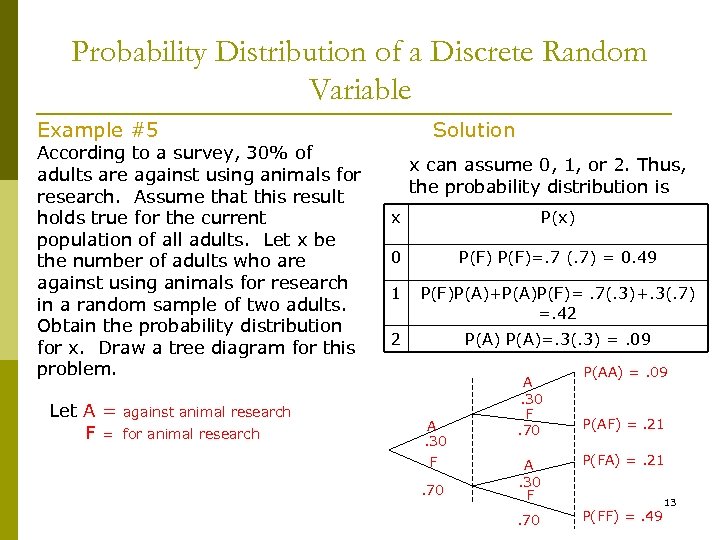
Probability Distribution of a Discrete Random Variable Example #5 According to a survey, 30% of adults are against using animals for research. Assume that this result holds true for the current population of all adults. Let x be the number of adults who are against using animals for research in a random sample of two adults. Obtain the probability distribution for x. Draw a tree diagram for this problem. Let A = F= against animal research for animal research Solution x can assume 0, 1, or 2. Thus, the probability distribution is x P(x) 0 P(F)=. 7 (. 7) = 0. 49 1 P(F)P(A)+P(A)P(F)=. 7(. 3)+. 3(. 7) =. 42 2 P(A)=. 3(. 3) =. 09 A. 30 F. 70 P(AA) =. 09 P(AF) =. 21 A. 30 F P(FA) =. 21 . 70 P(FF) =. 49 13
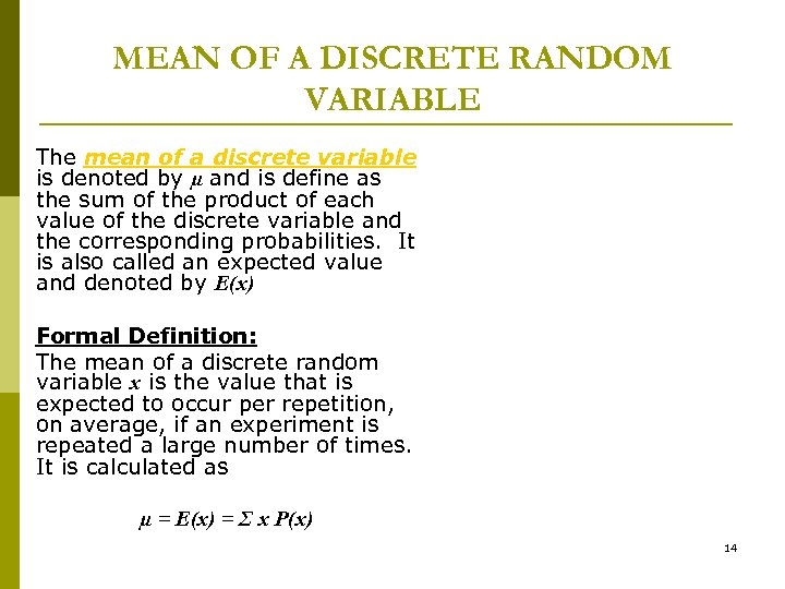
MEAN OF A DISCRETE RANDOM VARIABLE The mean of a discrete variable is denoted by µ and is define as the sum of the product of each value of the discrete variable and the corresponding probabilities. It is also called an expected value and denoted by E(x) Formal Definition: The mean of a discrete random variable x is the value that is expected to occur per repetition, on average, if an experiment is repeated a large number of times. It is calculated as µ = E(x) = Σ x P(x) 14
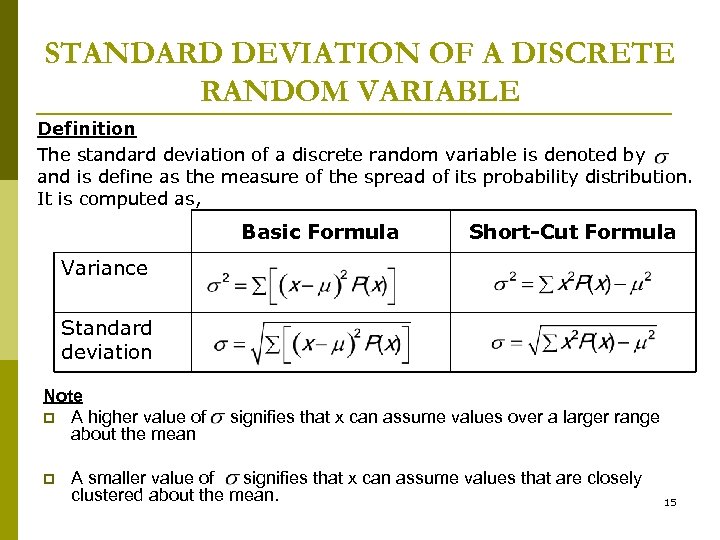
STANDARD DEVIATION OF A DISCRETE RANDOM VARIABLE Definition The standard deviation of a discrete random variable is denoted by and is define as the measure of the spread of its probability distribution. It is computed as, Basic Formula Short-Cut Formula Variance Standard deviation Note p A higher value of about the mean p signifies that x can assume values over a larger range A smaller value of signifies that x can assume values that are closely clustered about the mean. 15
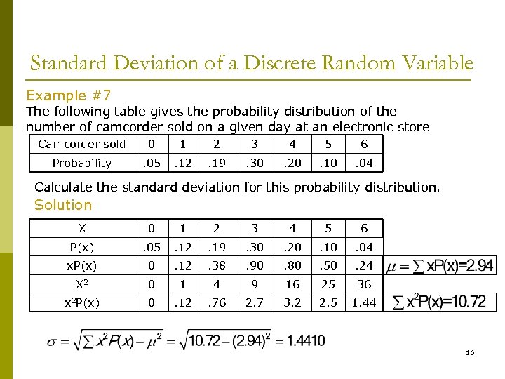
Standard Deviation of a Discrete Random Variable Example #7 The following table gives the probability distribution of the number of camcorder sold on a given day at an electronic store Camcorder sold 0 1 2 3 4 5 6 Probability . 05 . 12 . 19 . 30 . 20 . 10 . 04 Calculate the standard deviation for this probability distribution. Solution X 0 1 2 3 4 5 6 P(x) . 05 . 12 . 19 . 30 . 20 . 10 . 04 x. P(x) 0 . 12 . 38 . 90 . 80 . 50 . 24 X 2 0 1 4 9 16 25 36 x 2 P(x) 0 . 12 . 76 2. 7 3. 2 2. 5 1. 44 16
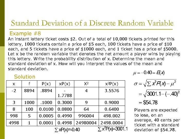
Standard Deviation of a Discrete Random Variable Example #8 An instant lottery ticket costs $2. Out of a total of 10, 000 tickets printed for this lottery, 1000 tickets contain a price of $5 each, 100 tickets have a price of $10 each, and 5 tickets have a price of $1000 each, and 1 ticket has a price of $5000. Let x be the random variable that denotes the net amount a player wins by playing this lottery. Write the probability distribution of x. Determine the mean and standard deviation of x. How will you interpret the values of the mean and standard deviation. Solution x f P(x) x. P(x) X 2 x 2 P(x) -2 8894 1. 7788 4 3. 5576 3 1000 0. 3000 9 0. 9000 8 100 0. 0800 64 0. 6400 998 5 0. 0005 0. 4990 996004 498. 002 4998 1 0. 0001 0. 4998 24980004 2498. 0004 Players are expected to lose, on an average, 40 cents per ticket with a standard 17 deviation of $54. 78.
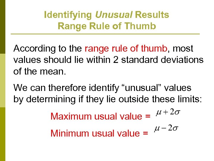
Identifying Unusual Results Range Rule of Thumb According to the range rule of thumb, most values should lie within 2 standard deviations of the mean. We can therefore identify “unusual” values by determining if they lie outside these limits: Maximum usual value = Minimum usual value =
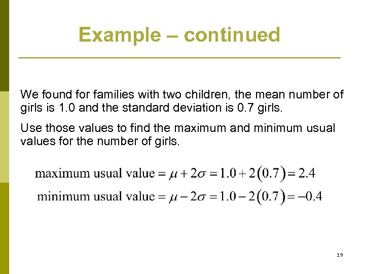
Example – continued We found for families with two children, the mean number of girls is 1. 0 and the standard deviation is 0. 7 girls. Use those values to find the maximum and minimum usual values for the number of girls. 19
Identifying Unusual Results Probabilities Rare Event Rule for Inferential Statistics If, under a given assumption (such as the assumption that a coin is fair), the probability of a particular observed event (such as 992 heads in 1000 tosses of a coin) is extremely small, we conclude that the assumption is probably not correct. 20
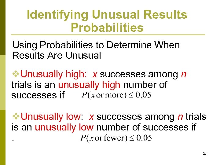
Identifying Unusual Results Probabilities Using Probabilities to Determine When Results Are Unusual v. Unusually high: x successes among n trials is an unusually high number of successes if. v. Unusually low: x successes among n trials is an unusually low number of successes if. 21
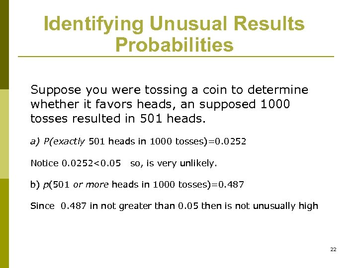
Identifying Unusual Results Probabilities Suppose you were tossing a coin to determine whether it favors heads, an supposed 1000 tosses resulted in 501 heads. a) P(exactly 501 heads in 1000 tosses)=0. 0252 Notice 0. 0252<0. 05 so, is very unlikely. b) p(501 or more heads in 1000 tosses)=0. 487 Since 0. 487 in not greater than 0. 05 then is not unusually high 22
fefa75d0ca0f0685a690f44f6da3ce57.ppt