2e57529f0cadedbe46fa8b001c8dc485.ppt
- Количество слайдов: 38
Chapter 5 Bitmapped Images Multimedia Systems
Key Points n n n For displayed images, physical dimension = pixel dimension/device resolution. To display an image at its natural size it is scaled by device resolution/image resolution. Downsampled images may look better than images stored at device resolution.
Key Points n n n Lossless compression: no information is lost during a compression/decompression cycle. Lossy compression: some information is discarded during the compression process. Run-length encoding (RLE), Huffman encoding, and LZ 77, LZ 78 and LZW are lossless methods. GIFs use LZW. JPEG compression is based on the use of the Discrete Cosine Transform (DCT). It is the most important lossy method for images.
Key Points n n GIFs are best for simple shapes with areas of flat colour. JPEGs are best for photographs and other images with continuous tones. Selecting an area of pixels defines a mask which protects the rest of the image from changes that are applied. A grey-scale mask is called an alpha channel and can be used for feathering and compositing, amongst other things. Pixel point processing: for a pixel with value p, we compute a new value p' = f(p). Brightness and contrast adjustments are common examples of pixel point processing.
Key Points n n Pixel group processing is based on a convolution process that also takes account of the values of neighboring pixels. Filters such as blurring and sharpening are the typical applications of pixel group processing. In general, applying geometrical transformations to bitmapped images requires interpolation of pixels and may cause a loss of image quality.
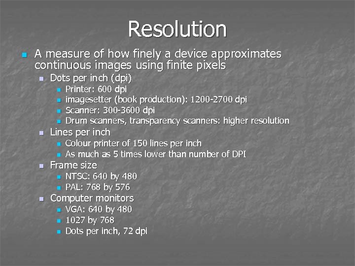
Resolution n A measure of how finely a device approximates continuous images using finite pixels n Dots per inch (dpi) n n n Lines per inch n n n Colour printer of 150 lines per inch As much as 5 times lower than number of DPI Frame size n n n Printer: 600 dpi imagesetter (book production): 1200 -2700 dpi Scanner: 300 -3600 dpi Drum scanners, transparency scanners: higher resolution NTSC: 640 by 480 PAL: 768 by 576 Computer monitors n n n VGA: 640 by 480 1027 by 768 Dots per inch, 72 dpi
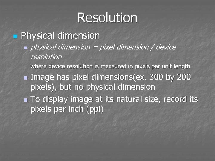
Resolution n Physical dimension n physical dimension = pixel dimension / device resolution where device resolution is measured in pixels per unit length Image has pixel dimensions(ex. 300 by 200 pixels), but no physical dimension n To display image at its natural size, record its pixels per inch (ppi) n
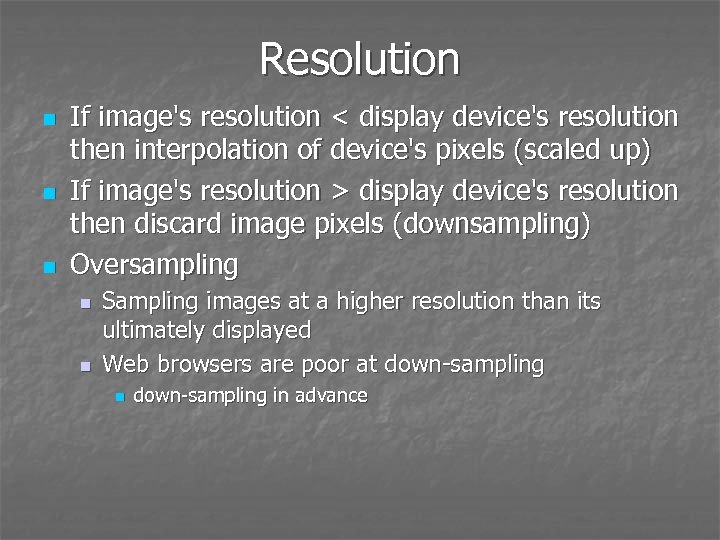
Resolution n If image's resolution < display device's resolution then interpolation of device's pixels (scaled up) If image's resolution > display device's resolution then discard image pixels (downsampling) Oversampling n n Sampling images at a higher resolution than its ultimately displayed Web browsers are poor at down-sampling n down-sampling in advance
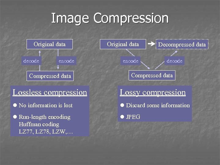
Image Compression Original data decode encode Original data encode Decompressed data decode Compressed data Lossless compression Lossy compression l No information is lost l Discard some information l Run-length encoding Huffman coding LZ 77, LZ 78, LZW, … l JPEG
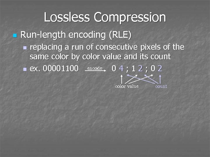
Lossless Compression n Run-length encoding (RLE) replacing a run of consecutive pixels of the same color by color value and its count encode n ex. 00001100 04; 12; 02 n color value count
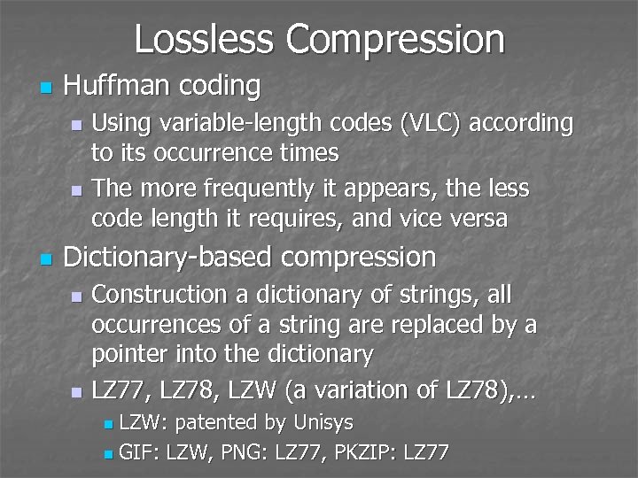
Lossless Compression n Huffman coding Using variable-length codes (VLC) according to its occurrence times n The more frequently it appears, the less code length it requires, and vice versa n n Dictionary-based compression Construction a dictionary of strings, all occurrences of a string are replaced by a pointer into the dictionary n LZ 77, LZ 78, LZW (a variation of LZ 78), … n LZW: patented by Unisys n GIF: LZW, PNG: LZ 77, PKZIP: LZ 77 n
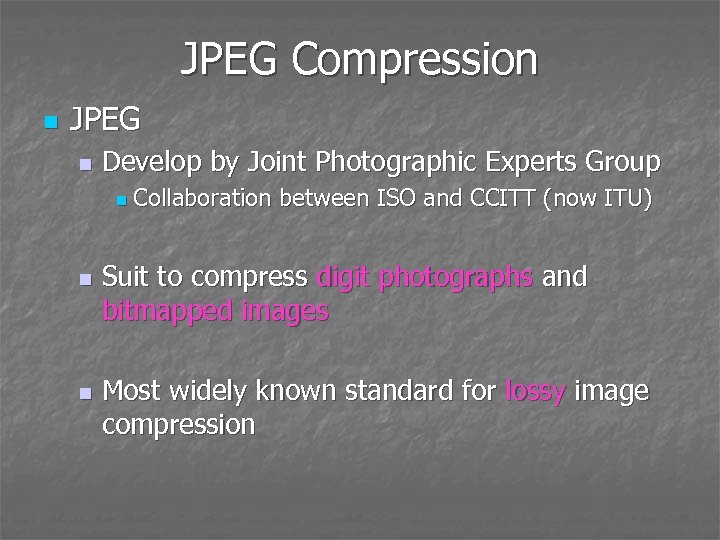
JPEG Compression n JPEG n Develop by Joint Photographic Experts Group n n n Collaboration between ISO and CCITT (now ITU) Suit to compress digit photographs and bitmapped images Most widely known standard for lossy image compression
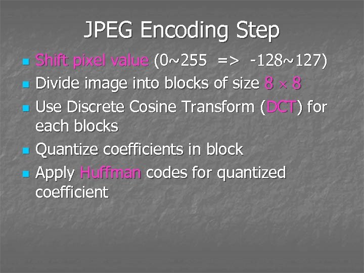
JPEG Encoding Step n n n Shift pixel value (0~255 => -128~127) Divide image into blocks of size 8 8 Use Discrete Cosine Transform (DCT) for each blocks Quantize coefficients in block Apply Huffman codes for quantized coefficient
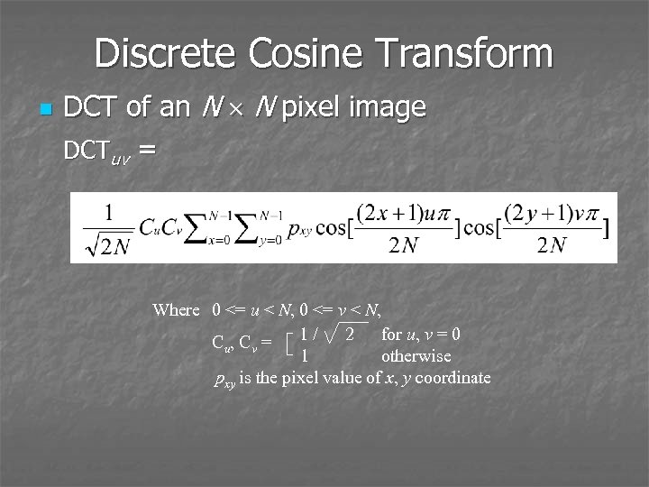
Discrete Cosine Transform n DCT of an N N pixel image DCTuv = Where 0 <= u < N, 0 <= v < N, 1/ 2 for u, v = 0 Cu, Cv = 1 otherwise pxy is the pixel value of x, y coordinate
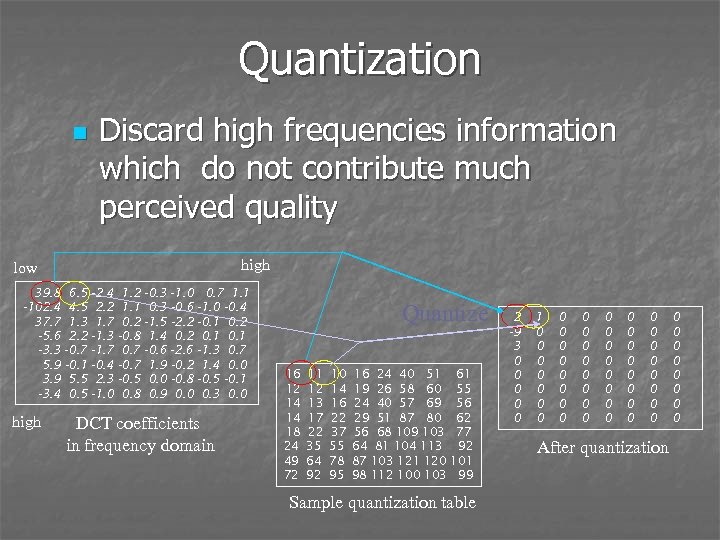
Quantization n Discard high frequencies information which do not contribute much perceived quality high low 39. 8 6. 5 -2. 4 -102. 4 4. 5 2. 2 37. 7 1. 3 1. 7 -5. 6 2. 2 -1. 3 -3. 3 -0. 7 -1. 7 5. 9 -0. 1 -0. 4 3. 9 5. 5 2. 3 -3. 4 0. 5 -1. 0 high 1. 2 -0. 3 -1. 0 0. 7 1. 1 0. 3 -0. 6 -1. 0 -0. 4 0. 2 -1. 5 -2. 2 -0. 1 0. 2 -0. 8 1. 4 0. 2 0. 1 0. 7 -0. 6 -2. 6 -1. 3 0. 7 -0. 7 1. 9 -0. 2 1. 4 0. 0 -0. 5 0. 0 -0. 8 -0. 5 -0. 1 0. 8 0. 9 0. 0 0. 3 0. 0 DCT coefficients in frequency domain Quantize 16 12 14 14 18 24 49 72 11 12 13 17 22 35 64 92 10 14 16 22 37 55 78 95 16 24 40 51 19 26 58 60 24 40 57 69 29 51 87 80 56 68 109 103 64 81 104 113 87 103 121 120 98 112 100 103 61 55 56 62 77 92 101 99 Sample quantization table 2 -9 3 0 0 0 1 0 0 0 0 0 0 0 0 0 0 0 0 After quantization 0 0 0 0
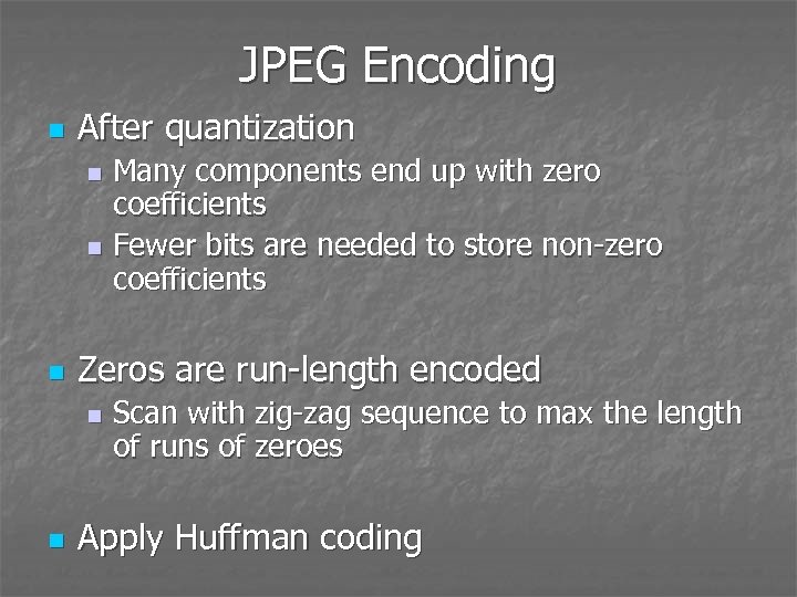
JPEG Encoding n After quantization Many components end up with zero coefficients n Fewer bits are needed to store non-zero coefficients n n Zeros are run-length encoded n n Scan with zig-zag sequence to max the length of runs of zeroes Apply Huffman coding
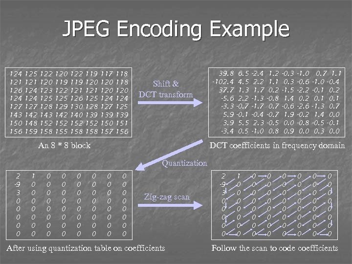
JPEG Encoding Example 124 121 126 124 127 143 150 156 125 121 124 127 142 148 159 122 120 123 125 128 143 152 158 120 119 122 125 129 142 155 122 119 121 126 130 140 152 158 119 120 121 125 128 139 152 158 117 120 124 127 139 150 157 118 120 124 125 139 151 156 Shift & DCT transform An 8 * 8 block 39. 8 -102. 4 37. 7 -5. 6 -3. 3 5. 9 3. 9 -3. 4 6. 5 4. 5 1. 3 2. 2 -0. 7 -0. 1 5. 5 0. 5 -2. 4 2. 2 1. 7 -1. 3 -1. 7 -0. 4 2. 3 -1. 0 1. 2 1. 1 0. 2 -0. 8 0. 7 -0. 5 0. 8 -0. 3 -1. 5 1. 4 -0. 6 1. 9 0. 0 0. 9 -1. 0 -0. 6 -2. 2 0. 2 -2. 6 -0. 2 -0. 8 0. 0 0. 7 1. 1 -1. 0 -0. 4 -0. 1 0. 2 0. 1 -1. 3 0. 7 1. 4 0. 0 -0. 5 -0. 1 0. 3 0. 0 DCT coefficients in frequency domain Quantization 2 -9 3 0 0 0 1 0 0 0 0 0 0 0 0 0 0 0 0 0 0 Zig-zag scan After using quantization table on coefficients 2 -9 3 0 0 0 1 0 0 0 0 0 0 0 0 0 0 0 0 0 0 Follow the scan to code coefficients
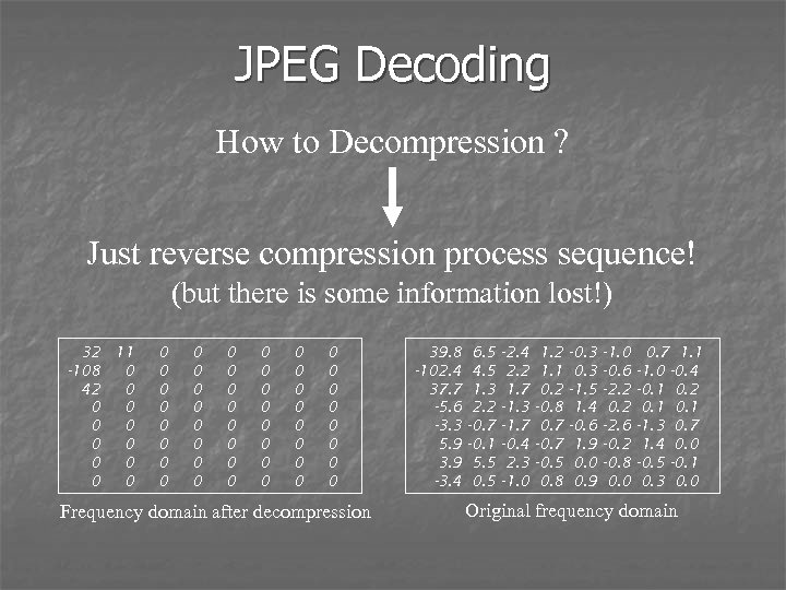
JPEG Decoding How to Decompression ? Just reverse compression process sequence! (but there is some information lost!) 32 11 -108 0 42 0 0 0 0 0 0 0 0 0 0 0 0 0 0 0 Frequency domain after decompression 39. 8 -102. 4 37. 7 -5. 6 -3. 3 5. 9 3. 9 -3. 4 6. 5 4. 5 1. 3 2. 2 -0. 7 -0. 1 5. 5 0. 5 -2. 4 2. 2 1. 7 -1. 3 -1. 7 -0. 4 2. 3 -1. 0 1. 2 1. 1 0. 2 -0. 8 0. 7 -0. 5 0. 8 -0. 3 -1. 5 1. 4 -0. 6 1. 9 0. 0 0. 9 -1. 0 -0. 6 -2. 2 0. 2 -2. 6 -0. 2 -0. 8 0. 0 0. 7 1. 1 -1. 0 -0. 4 -0. 1 0. 2 0. 1 -1. 3 0. 7 1. 4 0. 0 -0. 5 -0. 1 0. 3 0. 0 Original frequency domain
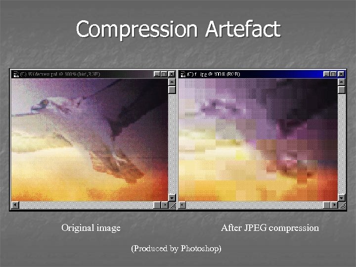
Compression Artefact Original image After JPEG compression (Produced by Photoshop)
Image Manipulation n Why manipulate image? n Correct deficiencies caused by creation or digitization n n Create unnatural image n n ex. Red-eye removal ex. Creating a glow around an object Image manipulation program n Adobe Photoshop, Photo. Impact
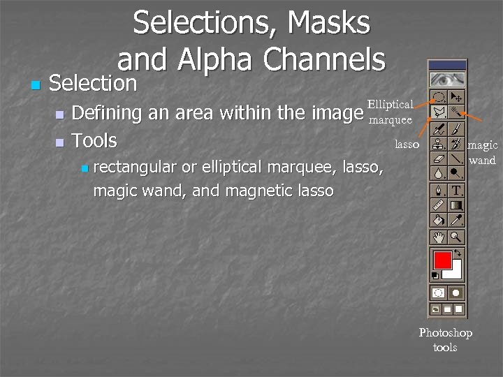
n Selections, Masks and Alpha Channels Selection Defining an area within the n Tools n n Elliptical image marquee rectangular or elliptical marquee, lasso, magic wand, and magnetic lasso magic wand Photoshop tools
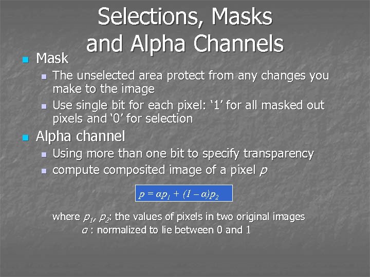
n Mask n n n Selections, Masks and Alpha Channels The unselected area protect from any changes you make to the image Use single bit for each pixel: ‘ 1’ for all masked out pixels and ‘ 0’ for selection Alpha channel n n Using more than one bit to specify transparency compute composited image of a pixel p p = αp 1 + (1 – α)p 2 where p 1, p 2: the values of pixels in two original images α : normalized to lie between 0 and 1
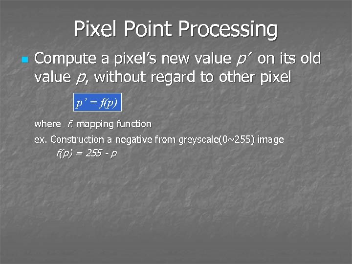
Pixel Point Processing n Compute a pixel’s new value p’ on its old value p, without regard to other pixel p’ = f(p) where f: mapping function ex. Construction a negative from greyscale(0~255) image f(p) = 255 - p
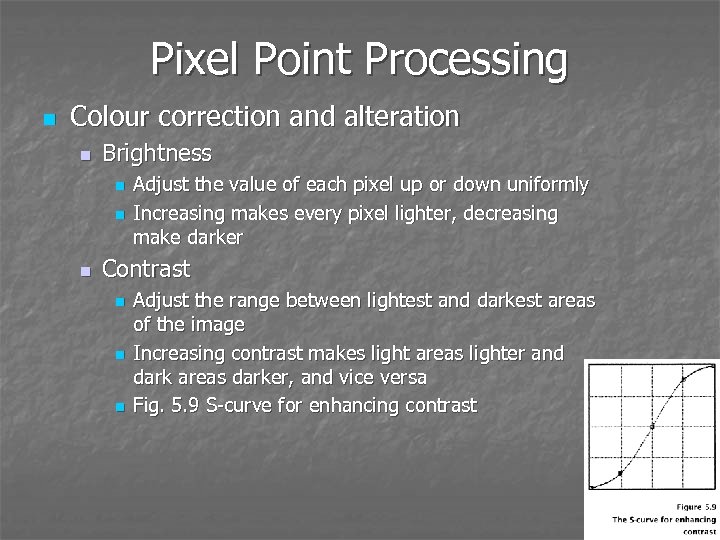
Pixel Point Processing n Colour correction and alteration n Brightness n n n Adjust the value of each pixel up or down uniformly Increasing makes every pixel lighter, decreasing make darker Contrast n n n Adjust the range between lightest and darkest areas of the image Increasing contrast makes light areas lighter and dark areas darker, and vice versa Fig. 5. 9 S-curve for enhancing contrast
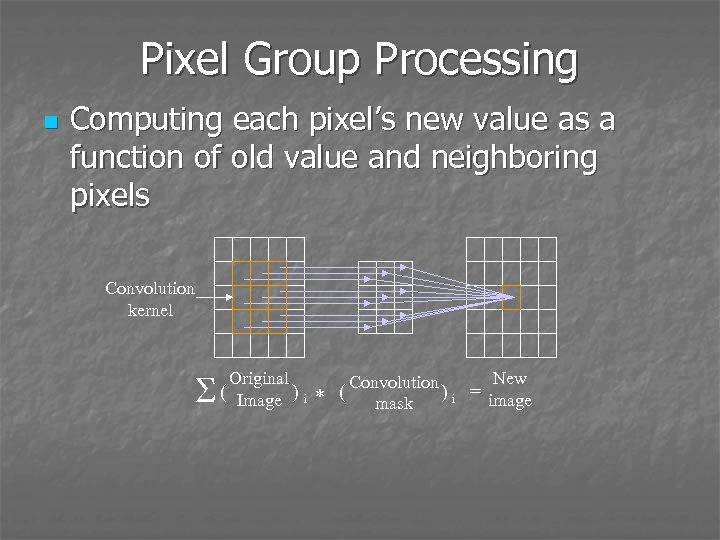
Pixel Group Processing n Computing each pixel’s new value as a function of old value and neighboring pixels Convolution kernel S Original ( Image ) i * ( New Convolution ) i = image mask
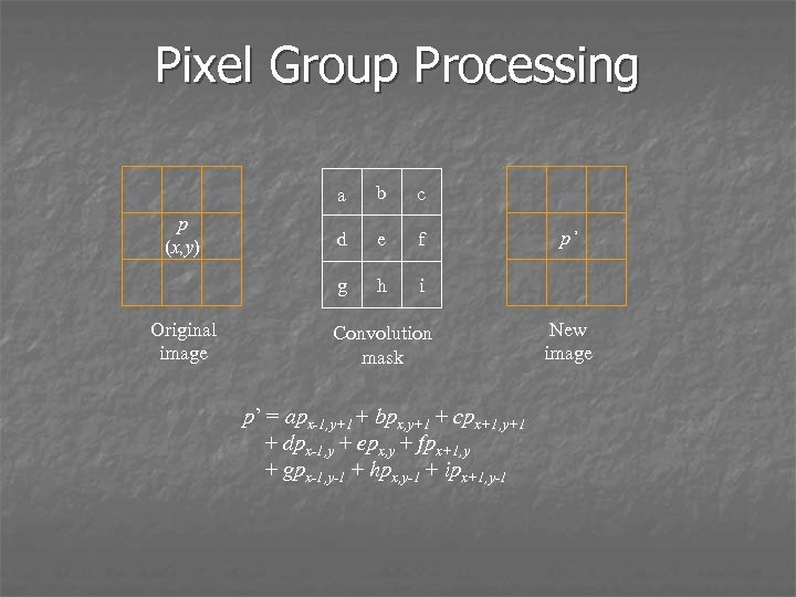
Pixel Group Processing a Original image c d e f g p (x, y) b h i Convolution mask p’ = apx-1, y+1 + bpx, y+1 + cpx+1, y+1 + dpx-1, y + epx, y + fpx+1, y + gpx-1, y-1 + hpx, y-1 + ipx+1, y-1 p’ New image
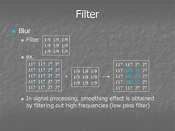
Filter n Blur n n Filter 1/9 1/9 ex. 117 117 117 n 1/9 1/9 1/9 117 117 117 27 27 27 * 1/9 1/9 1/9 117 117 117 105 105 117 27 57 57 57 27 27 27 In signal processing, smoothing effect is obtained by filtering out high frequencies (low pass filter)
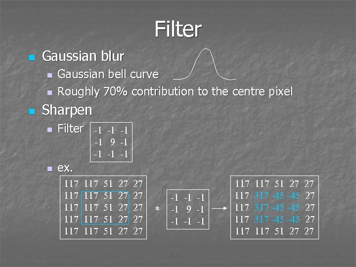
Filter n Gaussian blur n n n Gaussian bell curve Roughly 70% contribution to the centre pixel Sharpen n Filter -1 -1 9 -1 -1 n ex. 117 117 117 51 51 51 27 27 27 * -1 -1 9 -1 -1 117 117 117 51 27 317 -45 -45 317 -45 117 51 27 27 27
Filter n Unsharp masking Accentuate the edges, but retain the other parts n Idea n Blurring filters out high frequencies n If remove blurred image away from origin, it left high frequencies – the sharp edges n n Step Copy original image, applying a Gaussian blur to it n Subtracting the blurred mask pixel value from original pixel value with scaling factor n
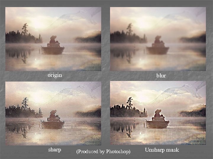
origin sharp blur (Produced by Photoshop) Unsharp mask
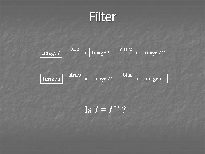
Filter Image I blur sharp Image I’ sharp blur Is I = I’’ ? Image I’’
Geometrical Transformations n n Scaling, translation, reflection, rotation and shearing Two transformation schemes n Forward mapping n n Assign original pixel value to transformed pixel Inverse mapping For each transformed pixel, find its inverse pixel value in original image n Advantage n n n No missing pixels Disadvantage n Require inverse mapping
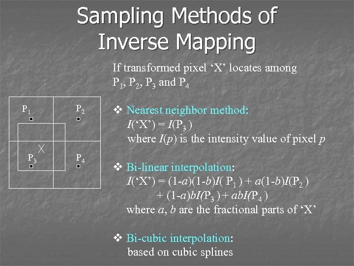
Sampling Methods of Inverse Mapping If transformed pixel ‘X’ locates among P 1, P 2, P 3 and P 4 P 1 P 3 P 2 P 4 v Nearest neighbor method: I(‘X’) = I(P 3 ) where I(p) is the intensity value of pixel p v Bi-linear interpolation: I(‘X’) = (1 -a)(1 -b)I( P 1 ) + a(1 -b)I(P 2 ) + (1 -a)b. I(P 3 ) + ab. I(P 4 ) where a, b are the fractional parts of ‘X’ v Bi-cubic interpolation: based on cubic splines
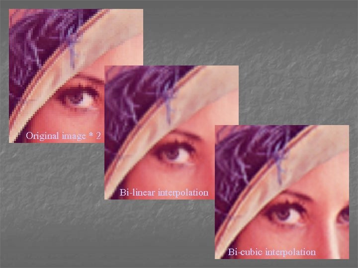
Original image * 2 Bi-linear interpolation Bi-cubic interpolation
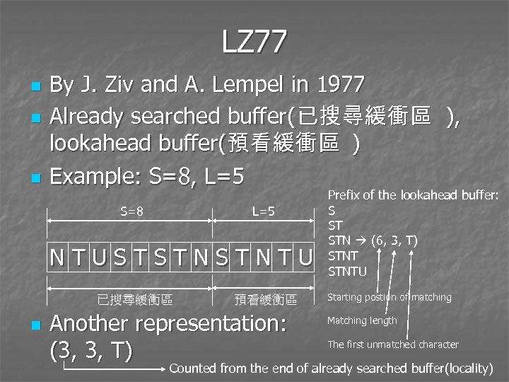
LZ 77 n n n By J. Ziv and A. Lempel in 1977 Already searched buffer(已搜尋緩衝區 ), lookahead buffer(預看緩衝區 ) Example: S=8, L=5 S=8 L=5 NTUSTSTNSTNTU 已搜尋緩衝區 n 預看緩衝區 Another representation: (3, 3, T) Prefix of the lookahead buffer: S ST STN (6, 3, T) STNTU Starting postion of matching Matching length The first unmatched character Counted from the end of already searched buffer(locality)

LZB n n n LZ 77: fixed length encoding, the matching for prefix is time-consuming LZB: variable length encoding Example, assume S<=8, T[0… 11]= NTUSTUSTUNTU NTUS input string already searched buffer after reading four characters Starting postition Because T[4… 8]=T[1… 5] use (01, 100) to encode “TUSTU” Matching length TUSTUSTUN Output “N” directly Output “TU” as (010, 010)
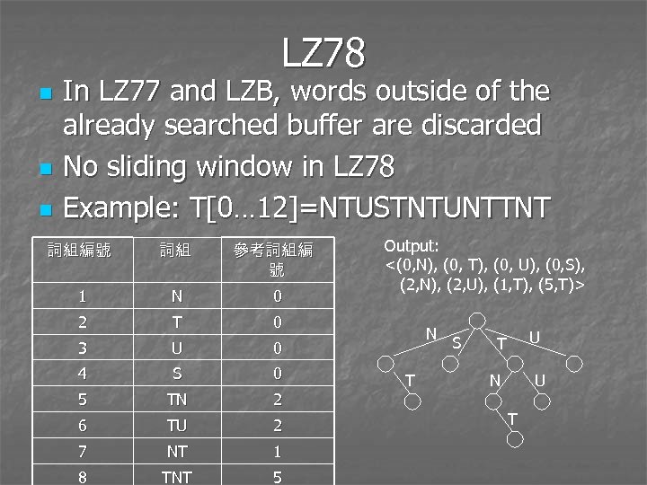
LZ 78 n n n In LZ 77 and LZB, words outside of the already searched buffer are discarded No sliding window in LZ 78 Example: T[0… 12]=NTUSTNTUNTTNT 詞組編號 詞組 參考詞組編 號 1 N 0 2 T 0 3 U 0 4 S 0 5 TN 2 6 TU 2 7 NT 1 8 TNT 5 Output: <(0, N), (0, T), (0, U), (0, S), (2, N), (2, U), (1, T), (5, T)> N T S U T N U T
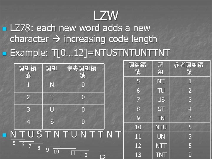
LZW n n LZ 78: each new word adds a new character increasing code length Example: T[0… 12]=NTUSTNTUNTTNT N 2 T 3 U 4 S NTUSTNTUNTTNT 5 6 7 8 9 10 11 12 13 TU 2 US 3 ST 4 9 0 1 8 0 NT 7 0 參考詞組編 號 6 0 詞 組 5 參考詞組編 號 1 n 詞組 詞組編 號 TN 2 10 NTU 5 11 UN 3 12 詞組編 號 NTT 5 13 TNT 9
2e57529f0cadedbe46fa8b001c8dc485.ppt