Chapter 5 Risk and Return.pptx
- Количество слайдов: 58


Chapter 5: “Basics of Risk and Return” Source Book: Essentials of Investment, 7 th edition. Source Book: Essentials of Investment Zvi Bodie, Alex Kane, Alan J. Marcus Prepared by: Ilyas Imachikov

For a typical person living in Almaty: • A time deposit in a commercial bank • A mutual fund, although not popular still • Real estate • Personal business • Automobile (even though not a profitable investment) Every individual security has its own risk and return characteristics; But should be judged on its contributions to both the expected return and the risk of the entire portfolio. However, from the standpoint of a professional – we have a much wider array of possible instruments: • Stocks • Bonds • Real estate • Precious metals • Collectibles • Options • Futures • Other derivative securities In this chapter we are going to look at the ABC of the risk and return which will help us in understanding the portfolio management process.

A key measure of investors’ success is the rate at which their funds have grown during the investment period. Holding-period return (HPR) – rate of return over a given investment period HPR may be recalculated to APR or some any other measure of rate of return. But don’t misinterpret it. HPR is a broader definition. Ex: The HPR of a share of stock depends on 1. Capital Gain / Price appreciation - the increase (or decrease) in the price of a share over the investment period as well as on 2. Dividend Yield / Dividends received - any dividend income the share has provided. The HPR of a bond depends on 1. Capital Gain / Price appreciation - the increase (or decrease) in the price of a bond over the investment period as well as on 2. Interest Yield / Coupons received– interest received in form of coupons on the bond If you purchase the bond at its face value and hold it till maturity → then Price Appreciation = 0

Note: The definition ignores the pattern and timing of payments. Ex: it doesn’t take into account the reinvestment income between the receipt of the dividend and the end of a holding period. This is usually important in valuation of bonds and other fixed-rate investments. Ex: ___________________________________ Suppose you are considering investing some of your money, now all invested in a bank account, in a stock market index fund. The price of a share in the fund is currently $100, and your time horizon is one year. You expect the cash dividend during the year to be $4. You expect the price per share after one year at $110. • Calculate the expected HPR For the Holding • Calculate the expected Capital Gain Period of one year • Calculate the expected Dividend Yield

Note: The definition ignores the pattern and timing of payments. Ex: it doesn’t take into account the reinvestment income between the receipt of the dividend and the end of a holding period. This is usually important in valuation of bonds and other fixed-rate investments. Ex: ___________________________________ Suppose you are considering investing some of your money, now all invested in a bank account, in a stock market index fund. The price of a share in the fund is currently $100, and your time horizon is one year. You expect the cash dividend during the year to be $4. You expect the price per share after one year at $110. • Calculate the expected HPR For the Holding • Calculate the expected Capital Gain Yield Period of one year • Calculate the expected Dividend Yield Capital Gain Yield Dividend Yield

Ex: ___________________________________ Suppose you are considering investing some of your money, now all invested in a bank account, in a stock market index fund. The price of a share in the fund is currently $100, and your time horizon is one year. You expect the cash dividend during the year to be $4. You expect the price per share after one year at $110. • Calculate the expected HPR For the Holding • Calculate the expected Capital Gain Yield Period of one year • Calculate the expected Dividend Yield Capital Gain Yield Dividend Yield HPR

The holding period return is a simple and unambiguous measure of investment return over a single period. But often you will be interested in average returns over longer periods of time. Ex: Consider a fund that starts with $1 mln under management at the beginning of the year. The fund receives additional funds to invest from new and existing, and also receives requests for redemptions from existing shareholders. Its net cash flow can be positive or negative. Table 5. 1 Quarterly cash flows and rates of return of a Assets under management at start of quarter ($ mln) mutual fund Holding-period return (%) 1 st Quarter 2 nd Quarter 3 rd Quarter 4 th Quarter 1, 0 1, 2 2, 0 0, 8 10, 0% 25, 0% -20, 0% 25, 0% Total assets before net inflows ($ mln) 1, 1 1, 5 1, 6 1, 0 Net Inflow ($ mln)* 0, 1 0, 5 -0, 8 0, 0 Assets under management at end of quarter ($ mln) 1, 2 2, 0 0, 8 1, 0 *New investment less redemptions and distributions, all assumed to occur at the end of each quarter How would we characterize fund performance over the year, given that fund experienced both cash inflows and outflows? We have three possible measures Arithmetic Average Geometric Average Dollar Weighted Return • Each measure has its advantages and shortcomings • Measures may vary considerably, so it’s important to understand their differences.

Arithmetic Average Table 5. 1 Quarterly cash flows and rates of return of a Assets under management at start of quarter ($ mln) mutual fund Holding-period return (%) The sum of returns in each period divided by the number of periods For our example the arithmetic average return would be: 1 st Quarter 2 nd Quarter 3 rd Quarter 4 th Quarter 1, 0 1, 2 2, 0 0, 8 10, 0% 25, 0% -20, 0% 25, 0% Total assets before net inflows ($ mln) 1, 1 1, 5 1, 6 1, 0 Net Inflow ($ mln)* 0, 1 0, 5 -0, 8 0, 0 Assets under management at end of quarter ($ mln) 1, 2 2, 0 0, 8 1, 0 *New investment less redemptions and distributions, all assumed to occur at the end of each quarter (10+25+20+25)/4 = 10% Shortcomings • This statistics ignores compounding thus doesn’t represent an equivalent, single quarterly rate for the year. Advantages • The arithmetic average is a useful forecast of performance in future quarters (iff the sample is large enough or representative enough to make accurate forecasts)

Geometric Average Table 5. 1 Quarterly cash flows and rates of return of a Assets under management at start of quarter ($ mln) mutual fund Holding-period return (%) The single perperiod return that gives the same cumulative performance as the sequence of actual returns In calculating the geometric average return we use compounding 1 st Quarter 2 nd Quarter 3 rd Quarter 4 th Quarter 1, 0 1, 2 2, 0 0, 8 10, 0% 25, 0% -20, 0% 25, 0% Total assets before net inflows ($ mln) 1, 1 1, 5 1, 6 1, 0 Net Inflow ($ mln)* 0, 1 0, 5 -0, 8 0, 0 Assets under management at end of quarter ($ mln) 1, 2 2, 0 0, 8 1, 0 *New investment less redemptions and distributions, all assumed to occur at the end of each quarter Geometric average return (1+0. 10)×(1+0. 25) ×(1 -0. 20)×(1+0. 25) = (1+r. G)4 r. G = [(1+0. 10)×(1+0. 25) ×(1 -0. 20)×(1+0. 25)] 1/4 – 1 = 0. 0829 or 8. 29% Assets under management at start of quarter ($ mln) Holding-period return (%) Total assets before net inflows ($ mln) Net Inflow ($ mln)* Assets under management at end of quarter ($ mln) 1 st Quarter 1, 0 10, 0% 1, 1 2 nd Quarter 1, 1 25, 0% 1, 4 3 rd Quarter 1, 4 -20, 0% 1, 1 4 th Quarter 1, 1 25, 0% 1, 4 Assets under management at start of quarter ($ mln) Holding-period return (%) Total assets before net inflows ($ mln) Net Inflow ($ mln)* Assets under management at end of quarter ($ mln) 1 st Quarter 1, 0 8, 29% 1, 1 2 nd Quarter 1, 1 8, 29% 1, 2 3 rd Quarter 1, 2 8, 29% 1, 3 4 th Quarter 1, 3 8, 29% 1, 4 Notice the same performance for both cases

Geometric Average Table 5. 1 Quarterly cash flows and rates of return of a Assets under management at start of quarter ($ mln) mutual fund Holding-period return (%) The single perperiod return that gives the same cumulative performance as the 1 st sequence of actual Quarter 1, 0 returns 10, 0% 1, 1 0, 1 1, 2 1 st Quarter 2 nd Quarter 3 rd Quarter 4 th Quarter 1, 0 1, 2 2, 0 0, 8 10, 0% 25, 0% -20, 0% 25, 0% Total assets before net inflows ($ mln) 1, 1 1, 5 1, 6 1, 0 Net Inflow ($ mln)* 0, 1 0, 5 -0, 8 0, 0 Assets under management at end of quarter ($ mln) 1, 2 2, 0 0, 8 1, 0 *New investment less redemptions and distributions, all assumed to occur at the end of each quarter 2 nd Quarter 1, 2 25, 0% 1, 5 0, 5 2, 0 3 rd Quarter 2, 0 25, 0% 2, 5 -0, 8 1, 7 4 th Quarter 1, 7 -20, 0% 1, 4 0, 0 1, 4 1 st Quarter 1, 0 10, 0% 1, 1 0, 1 1, 2 2 nd Quarter 1, 2 -20, 0% 1, 0 0, 5 1, 5 3 rd Quarter 1, 5 25, 0% 1, 8 -0, 8 1, 0 4 th Quarter 1, 0 25, 0% 1, 3 0, 0 1, 3 1 st Quarter 1, 0 25, 0% 1, 3 0, 1 1, 4 2 nd Quarter 1, 4 -20, 0% 1, 1 0, 5 1, 6 3 rd Quarter 1, 6 10, 0% 1, 7 -0, 8 0, 9 In each case we will calculate the same geometric average return of 8, 29% 4 th Quarter 0, 9 25, 0% 1, 2 0, 0 1, 2 Shortcomings • The geometric average is often called a time-weighted average return because it doesn’t take into account variations in money under management in each quarter. In other words, it doesn’t take into account differences in customer deposits and withdrawals in and out of fund. Advantages • Makes a use of compounding thus does represent an equivalent, single quarterly rate of return for the year. → A good representative measure to evaluate past performance. • Sometimes we wish to ignore variations in money under management. • Ex: Published data on past returns earned by mutual funds are required to be time-weighted returns. • Logic is that as a fund manager doesn’t have a full control of the amount of funds under management, we should not weight returns in one period more heavily than those in other periods when assessing typical past performance.

Dollar Weighted Return The internal rate of return on an investment Table 5. 1 Quarterly cash flows and rates of return of a Assets under management at start of quarter ($ mln) mutual fund Holding-period return (%) 1 st Quarter 2 nd Quarter 3 rd Quarter 4 th Quarter 1, 0 1, 2 2, 0 0, 8 10, 0% 25, 0% -20, 0% 25, 0% Total assets before net inflows ($ mln) 1, 1 1, 5 1, 6 1, 0 Net Inflow ($ mln)* 0, 1 0, 5 -0, 8 0, 0 Assets under management at end of quarter ($ mln) 1, 2 2, 0 0, 8 1, 0 *New investment less redemptions and distributions, all assumed to occur at the end of each quarter When we wish to account for the varying amounts under management, we treat the fund cash flows to investors as we would a capital budgeting problem in corporate finance. 0 Net cash flow ($ mln) 1 Time 2 -1, 0 -0, 1 -0, 5 3 4 0, 8 1, 0 The project which needs cash outflows and provides cash inflows The IRR is the interest rate that sets the present value of the cash flows realized on the portfolio (including $1 mln liquidation value) equal to the initial cost of establishing the portfolio. The dollar weighted return in this example is less than the time-weighted return of 8. 29% because the portfolio returns were higher when less money was under management.

Shortly, how to use each ratio • The arithmetic average is a useful forecast of performance in future quarters (iff the sample is large enough or representative enough to make accurate forecasts) • Geometric average is a good representative measure to evaluate past performance. • When we wish to account for the varying amounts under management we may use dollar weighted average.

Shortly, how to use each ratio • The arithmetic average is a useful forecast of performance in future quarters (iff the sample is large enough or representative enough to make accurate forecasts) • Geometric average is a good representative measure to evaluate past performance. • When we wish to account for the varying amounts under management we may use dollar weighted average. Question • Assuming that our fund is going to attract some $400’ 000 and $300’ 000 in net cash inflows in quarters 1 and 2, respectively, of the next year. What dollar amount of assets under management should we expect at the end of each quarter, given the information provided from the table 5. 1?

Question • Assuming that our fund is going to attract some $400’ 000 and $300’ 000 in net cash inflows in quarters 1 and 2, respectively, of the next year. What dollar amount of assets under management should we expect at the end of each quarter, given the information provided from the table 5. 1? Assets under management at start of quarter ($ mln) 1 st 2 nd 3 rd 4 th 1 st 2 nd Quarter Quarter 1, 0 1, 2 2, 0 0, 8 1, 0 1, 5 10, 0% 25, 0% -20, 0% 25, 0% 10, 0% Total assets before net inflows ($ mln) 1, 1 1, 5 1, 6 1, 0 1, 1 1, 7 Net Inflow ($ mln)* 0, 1 0, 5 -0, 8 0, 0 0, 4 0, 3 Assets under management at end of quarter ($ mln) 1, 2 2, 0 0, 8 1, 0 1, 5 2, 0 Holding-period return (%)

From bank management we remember that there may be a lot of interest rate quotations, such as, Simple Interest, Discount Rate, APR, etc. The same is true for Quoting Rates of Return. How to report profitability of various investment instruments? Returns on assets with regular cash flows, such as mortgages (with monthly payments) and bonds (with semiannual coupons), usually are quoted as APRs. APR annualizes per-period rates using a simple interest approach, but ignores compounding of interest. We can translate APR into EAR by remembering that APR = Per-period rate × Periods per year 1 + EAR = (1 + Rate period)n We can retranslate the relationship between APR and EAR as follows: 1 + EAR = (1 + Rate period)n = (1 + APR/n)n APR = [(1+EAR)1/n – 1] × n The EAR diverges by greater amounts from the APR as n becomes larger (i. e. , as we compound cash flows more frequently). With continuous compounding (when n approaches to ∞) the relationship between the APR and EAR becomes 1+EAR = e. APR Or equivalently, APR = ln(1 + EAR)

Example: Annualizing Treasury-Bill Returns Suppose you buy a $10’ 000 face value Treasury bill maturing in one month for $9’ 900. On the bill’s maturity date, you collect the face value. • What is the HPR for this one-month investment? • What is the APR for this period? • What is the EAR? Compare this investment with the same T-bill but with face value of $100’ 000, maturing in three months and a current price of $97’ 059. • What is the HPR for this one-month investment? • What is the APR for this period? • What is the EAR? Why does the EAR differ in the two cases? Which investment has a higher EAR? Which investment looks to be more profitable?

$100’ 000 bill $10’ 000 bill Example: Annualizing Treasury-Bill Returns APR on this investment is = 1. 01 × 12 = 12. 12% 1+ EAR = (1. 0101)12 => EAR = 12. 82% APR on this investment is = 3. 03 × 12 = 12. 12% 1+ EAR = (1. 0303)4 = > EAR = 12. 68% Which investment has a higher EAR? $10’ 000 bill Which investment looks to be more profitable? $10’ 000 bill Why does the EAR differ in the two cases? Answer: Compounding

When we want to quantify risk regarding our expected HPR, we face two questions 1. What HPRs are possible? 2. How likely is each case? Scenario Analysis: 1. Devise a list of possible economic outcomes, or scenarios 2. Specify the likelihood of each scenario and the HPR the asset will realize in that scenario. The list of all possible HPRs with associated probabilities is called the probability distribution of HPRs. Consider an investment in a broad portfolio of stocks (say, an index fund) which we will refer to as the “stock market”. A very simple scenario analysis for the stock market (assuming only three possible scenarios) is illustrated in the table below: Table 5. 2 State of the Economy Probability Boom distribution of Normal growth HPR on the stock market Recession Scenario, s Probability, p(s) HPR 1 0. 25 44% 2 0. 50 14% 3 0. 25 -16%

Table 5. 2 State of the Economy Probability Boom distribution of Normal growth HPR on the stock market Recession Scenario, s Probability, p(s) HPR 1 0. 25 44% 2 0. 50 14% 3 0. 25 -16% The probability distribution helps us derive measurements for both the reward and the risk of the investment. Reward from the investment is its expected return, which you can think of as the average HPR you would earn if you were to repeat an investment in the asset many times. The general formula the expected return is: HPR in each Number of scenarios scenario Expected HPR Probability of each scenario Calculate the expected return on the stock market

Table 5. 2 State of the Economy Probability Boom distribution of Normal growth HPR on the stock market Recession Scenario, s Probability, p(s) HPR 1 0. 25 44% 2 0. 50 14% 3 0. 25 -16% The probability distribution helps us derive measurements for both the reward and the risk of the investment. Reward from the investment is its expected return, which you can think of as the average HPR you would earn if you were to repeat an investment in the asset many times. The general formula the expected return is: HPR in each Number of scenarios scenario Expected HPR Probability of each scenario Calculate the expected return on the stock market: E(r) = 0. 25× 44% + 0. 50× 14% + 0. 25×(-16%) = 14% Does the return we have calculated represent the actual return that we will have? Can we state that we will earn a 14% return on our investment in stocks? What is the possibility that there will be any deviation in actual return from our expected 14%?

Of course there is a risk to our investment and actual return may deviate from our expected 14%. • If a “boom” materializes actual return would be 44%, representing a 30% positive surprise. • In a recession the return may be disappointing -16%, representing a 30% negative surprise. Risk surrounding the investment is a function of the magnitudes of possible surprises. The measures of risk to be introduced is variance and standard deviation. • What these two measures tell us is by how much we can expect actual returns to be different from expected returns. • Formulas, you know them: For our example: What does this number tell us?

Drawback to the use of variance and standard deviation as a measures of risk: • treat positive and negative deviations symmetrically, whereas a risk is associated with negative deviations. • However, evidence shows that for fairly short holding periods, the returns of almost all diversified portfolios are well described by a normal distribution. • In conditions stated above we may use standard deviation as a measure of possible negative surprises. A share of stock of A-Star Inc. is now selling for $23. 50. A financial analyst summarizes the uncertainty about next year’s HPR on the stock by specifying three possible scenarios: Business conditions Scenario, s End-of- Annual Probability, p(s) Year price Dividend High growth 1 0. 35 $4. 40 Normal growth 2 0. 30 $27 $4. 00 No growth 3 0. 35 $15 $4. 00 • What are the annual HPRs of A-Star stock for each of the three scenarios? Calculate the expected HPR and the standard deviation of the HPR.

A share of stock of A-Star Inc. is now selling for $23. 50. A financial analyst summarizes the uncertainty about next year’s HPR on the stock by specifying three possible scenarios: Business conditions Scenario, s End-of- Annual Probability, p(s) Year price Dividend High growth 1 0. 35 $4. 40 Normal growth 2 0. 30 $27 $4. 00 No growth 3 0. 35 $15 $4. 00 • What are the annual HPRs of A-Star stock for each of the three scenarios? Calculate the expected HPR and the standard deviation of the HPR. Business conditions Probability, End-of-Year Annual Purchase Price Capital Total $ Scenario, s p(s) price Dividend of stock Gain Return HPR High growth 1 0, 35 $35, 00 $4, 40 $23, 50 $11, 50 $15, 90 67, 66% Normal growth 2 0, 30 $27, 00 $4, 00 $23, 50 $7, 50 31, 91% No growth 3 0, 35 $15, 00 $4, 00 $23, 50 -$8, 50 -$4, 50 -19, 15% E(r) = 0. 35× 67. 66% + 0. 30× 31. 91% + 0. 35×(-19. 15%) = 26. 55%

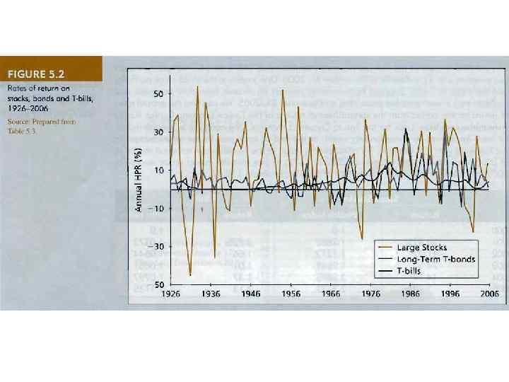
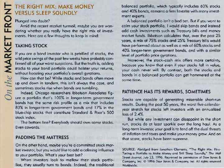
How much, if anything, should you invest in an index stock fund such as the one described in Table 5. 2? First, you must ask how much of an expected reward is offered to compensate for the risk involved in investing money in stocks? The reward for additional risk is measured as the difference between the expected HPR on the index stock fund and the risk-free rate (the rate you can earn by leaving money in risk-free assets such as T-bills, MMF, or the bank), and usually is named as the riskpremium. Ex: If the rf in the example is 6%, and the expected index fund return is 14%, then the risk premium on stocks is 8% per year. The degree to which investors are willing to commit funds to stocks depends on risk aversion. In theory then, there must always be a positive risk premium on stocks in order to induce risk-averse investors to hold the existing supply of stocks instead of placing them in riskfree assets. In fact, • In long term, most often, we may see that stock market returns are generally higher than bond market returns, with greater risks associated with those returns of course. • During bad times at stock market, we may see an outflow of capital from stock to bond markets, i. e. , reward for excessive risk drops, and thus people take their funds out to a safer place. This is a partly explanation of course. See the case below

Treasuries на грани фола Улучшение ситуации в экономике США и позитивные сигналы из ЕС привели к росту доходности US Treasuries Анна Королева Начало 2012 года может оказаться для американских казначейских облигаций самым худшим за последние девять лет на фоне признаков улучшения ситуации в экономике США, а также слухах, что Европа приблизилась к выходу из долгового кризиса. Улучшение ситуации в экономике США и позитивные сигналы из ЕС привели к росту доходности US Treasuries Фото: AP В пятницу доходность 10 -летних американских облигаций выросла на 5 базисных пунктов, до 2, 02%, согласно Bloomberg Bond Trader prices. Рост доходности 10 -летних US Treasuries связан со статистическими показателями, опубликованными в США. Так, данные по количеству обращений за пособием по безработице оказались лучше ожиданий, а продажи жилья выросли. На этом фоне инвесторы стали проявлять меньший интерес к активам-убежищам. «Происходят улучшения на рынке труда, – говорит Ричард Джилхули, стратег Toronto-Dominion Bank TD Securities Inc. в Нью-Йорке. – И как только мы получим хорошие статистические данные (в США) в первом квартале, увидим большой всплеск доходности Treasuries» . В последние дни действительно наметилось повышение доходности казначейских облигаций США, которые принято считать наименее рискованным инструментом на долговом рынке, отмечает ведущий аналитик ИФ «Олма» Антон Старцев. Так, доходность по 10 -летним казначейским облигациям превысила 2%, вернувшись к уровням декабря прошлого года. Одновременно начал сокращаться спред EMBI+, и это означает, что инвесторы увеличивают склонность к принятию риска. Примечательно, что доходности гособлигаций стран еврозоны в среднем сократились – европейский долговой сектор долгое время рассматривался как источник рисков, теперь же опасения смягчаются благодаря успешным размещениям суверенных облигаций стран еврозоны и поддержке ликвидности через механизм трехлетнего репо, предоставляемого ЕЦБ. К тому же греческие чиновники, по сообщениям зарубежных СМИ, завершают переговоры с кредиторами о реструктуризации государственного долга, что делает более привлекательными европейские облигации. Ситуация в США и Европе с экономической точки зрения различна, но с точки зрения воздействия на рынки и там есть основания для оптимизма, объясняет начальник отдела управления инвестициями и аналитической поддержки ИФК «Солид» Михаил Королюк. В США наблюдается ускорение экономического роста. Судя по всему, текущее состояние экономики неплохое, и рынкам пока этого достаточно для оптимизма. То, что этот экономический рост развился на «допинге» дефицита бюджета в 8% от ВВП, пока игнорируется. В Европе, напротив, экономика находится на грани рецессии, причем ряд стран уже отчетливо находятся в рецессии, а ряд оттуда и не вылезали уже по несколько лет. Однако оптимизм рынков связан с надеждами на то, что дно европейского кризиса уже пройдено или вот-вот будет пройдено, а рецессия будет недлинной и мягкой. В связи с этим инвесторы ожидают некоторого снижения доходности долговых бумаг, особенно с большими сроками до погашения, и перекладываются в бумаги короткой дюрации и/или акции. В целом это вполне разумное поведение. Обычно при резком падении акций цены на облигации растут, так как срабатывает эффект risk off (переток денег в наиболее безопасные активы), объясняет начальник управления финансовых рисков Абсолют банка Дмитрий Мурзинов. Впрочем, уточняет он, при росте рынка акций устойчивой корреляционной закономерности между этими двумя рынками не наблюдается, по крайней мере, в широком временном диапазоне. Что же касается нынешнего ценового падения на рынке облигаций при рекордно низких, по историческим меркам, доходностях, то любая позитивная статистика вызывает паническую реакцию со стороны нервничающих инвесторов. Однако, судя по динамике тех же самых макроэкономических индикаторов, дефляционная спираль, начавшаяся в 2008 году, все еще продолжает раскручиваться. И это происходит, несмотря на титанические усилия центральных банков, замещающих «сгоревший» кредит наличными деньгами. Пока процесс делевереджа частного сектора продолжается. Скорее всего, цены на высококачественные облигации будут оставаться высокими. Действительно, вряд ли ситуация со снижением цен на «защитные» облигации и, соответственно, ростом их доходности сохранится надолго. Инвесторам следует покупать Treasuries, так как существует вероятность их возвращения к уровню доходности 2, 05% в ближайшее время на фоне опасений, что Европа не в состоянии решить свой кризис суверенного долга, считает Ларри Мильштейн, управляющий директор R. W. Pressprich & Co. «Данные по США выглядят хорошо, – говорит он. – Но я все еще не убежден в них по отношению к Европе» . «Чем лучше настроения в Европе и ситуация в американской экономике, тем хуже Treasuries, – передает Bloomberg слова Кевина Фланагана, стратега Morgan Stanley Smith Barney. – Тем не менее существует значительная неопределенность, и, несмотря на положительные признаки, есть много нерешенных вопросов» . Эти прогнозы подтверждают эксперты Всемирного банка, которые заявили, что экономика США вырастет на 2, 2% в 2012 году, в то время как ВВП зоны евро сократится на 0, 3%. Данный прогноз значительно хуже того, который давала организация еще осенью. В целом же, подводит итог аналитик «Инвесткафе» Антон Сафонов, сейчас может быть хорошей идеей инвестировать в облигации крупнейших экономик, то есть как раз в защитные бумаги, так как при ухудшении ситуации в мировой экономике их доходность в дальнейшем будет расти, так как эти страны будут себя чувствовать все равно относительно стабильно и таким инвестициям ничего не угрожает. По материалам expert. ru «Expert Online» / 23 янв 2012, 14: 12

As an addition for your better understanding of stock and bond markets But don’t take this as a universe rule

For your understanding: Gilt-edged securities, or gilts, are bonds issued by the U. K. government. Similar to U. S. Treasury bonds, they are debt obligations with maturities ranging from 1 month to 30 years.

So, we will assume that the risk premium that an investor demands to hold a risky portfolio rather than placing all of her funds in safe T-bills offering the risk-free rate is proportional to the product of her risk aversion, A, and the variance of the risky portfolio’s rate of return : variance of the risky portfolio’s rate of return Risk premium Risk aversion Notes to the formula: • Investors would not demand a risk premium for a risk-free portfolio (for which = 0) • As the portfolio’s variance or an investor’s risk aversion increase, we need a higher risk premium to satisfy the investor for these two factors. • The factor of ½ is merely a scale factor. It is widely used by convention, but has no bearing on the analysis. • To use this equation, all rates of return must be expressed as decimals rather than percentages. • This model is a good thing to understand the factors affecting the risk premium. It may be impossible to use this model for analysis.

By examining risk-return trade-off offered by a representative portfolio (and willingly held by the representative investor) we should be able to infer something about the typical investor’s risk aversion. If investors trade off risk against return in the manner specified by the equation above, then we can infer the degree of risk aversion from the characteristics of the market portfolio, M, as: If risk premium is 8%, and the standard deviation is 20%, then we would infer risk aversion of this investor to be A = 0. 08/0. 202 = 2 In practice, • We cannot observe risk premium investors expect to earn on their investments. • We can only observe actual returns after the fact. • Different investors may have different expectations about the risk and return of various assets.

• The Sharpe ratio is used to characterize how well the return of an asset compensates the investor for the risk taken, the higher the Sharpe ratio number the better. • When comparing two assets each with the expected return E[R] against the same benchmark with return Rf, the asset with the higher Sharpe ratio gives more return for the same risk. • Investors are often advised to pick investments with high Sharpe ratios. However like any mathematical model it relies on the data being correct. Pyramid schemes with a long duration of operation would typically provide a high Sharpe ratio when derived from reported returns, but the inputs are false. • Sharpe ratios, along with Treynor ratios and Jensen's alphas, are often used to rank the performance of portfolio or mutual fund managers. • The Sharpe measure is applicable only to well diversified portfolios, such as S&P 500, or other widerange stock indices. Concept Check 5. 3 a. A respected analyst forecasts that the return of the S&P 500 Index portfolio over the coming year will be 10%. The one-year T-bill rate is 5%. Examination of recent returns of the S&P 500 Index suggest that the standard deviation of returns will be 18%. What does this information suggest about the degree of risk aversion of the average investor, assuming that the average portfolio resembles the S&P 500? b. What is the Sharpe measure of the portfolio in (a)?

Concept Check 5. 3 a. A respected analyst forecasts that the return of the S&P 500 Index portfolio over the coming year will be 10%. The one-year T-bill rate is 5%. Examination of recent returns of the S&P 500 Index suggest that the standard deviation of returns will be 18%. What does this information suggest about the degree of risk aversion of the average investor, assuming that the average portfolio resembles the S&P 500? b. What is the Sharpe measure of the portfolio in (a)? Answers: a. If the average investor chooses the S&P 500 portfolio, then the implied degree of risk aversion is given by “A”. What does the Sharpe ratio of 0. 28 tell us? b. It tells that over this year we may expect that, each increase in portfolio standard deviation of 1% will be rewarded by an increased risk premium of 0. 28%.


Example 5. 4: Historical Means and Standard Deviations Year 1 2 3 4 5 Total (1) Rate of Return 16, 9% 31, 3% -3, 2% 30, 7% 7, 7% 83, 4% In the table to the left you may see the rates of return for the S&P 500 portfolio. 1. Calculate average rate of return on the S&P 500 portfolio over the period of 5 years. 2. Calculate the standard deviation of returns for the period of these 5 years. (2) (1) (2) Deviation from (3) Rate of Deviation from Average Return Squared Return Average Return (in decimals) Deviation 16, 9% 0, 2 0, 0 31, 3% 14, 6 213, 2 -3, 2% -19, 9 396, 0 30, 7% 14, 0 196, 0 7, 7% -9, 0 81, 0 83, 4% 886, 2 Average rate of return = 83. 4/5 = 16. 7 Variance = 886. 2/(5 -1) = 221. 6 1. Calculate average rate of return (by the way, which average would you use? ) 2. Calculate deviation from average return. 3. Find variance. 4. Find standard deviation.

Example 5. 5: The Risk Premium and Growth of Wealth Consider two investors with $1 mln as of December 31, 2000. One invests in the small stock portfolio, and the other in T-bills. Suppose both investors reinvest all income from their portfolios and liquidate their investments five years later, on December 31, 2005. The annual rates of return for the 5 -year period is given in the table. 2001 2002 2003 2004 2005 Return on Small Stocks 28, 82% -11, 72% 74, 54% 14, 34% 3, 20% Return on T-bills 3, 72% 1, 66% 1, 01% 1, 37% 3, 13% These are actual rates of return on S&P 500 Index for the period of 2001 -2005 1. Calculate the amount of wealth for each portfolio at the end of each year. 2. Calculate the total dollar return for the five year period. 3. Suppose you put your money in a one-year bank account paying interest once at the end year, and revolve the account each year so that interest earned in a given year is reinvested in the next year, what should be the APR on the bank account be to provide you the same result as the two portfolios?

2000 2001 2002 2003 2004 2005 Small Stocks Return Wealth Index 1, 0000 28, 82% 1, 2882 -11, 72% 1, 1372 74, 54% 1, 9849 14, 34% 2, 2695 3, 20% 2, 3422 T-bills Return Wealth Index 1, 0000 3, 72% 1, 0372 1, 66% 1, 0544 1, 01% 1, 0651 1, 37% 1, 0797 3, 13% 1, 1135 Wealth of each portfolio: Small Stocks = $2’ 342’ 200 T-bills = $1’ 113’ 500 Total $ return of each portfolio: Small Stocks = $1’ 342’ 200 T-bills = $113’ 500 The difference in total return is dramatic!!! Suppose you put your money in a one-year bank account paying interest once at the end year, and revolve the account each year so that interest earned in a given year is reinvested in the next year, what should be the APR on the bank account be to provide you the same result as the two portfolios? Answer: to find this we can use the geometric average return: ____Small Stocks_______T-Bills______ The large difference in geometric average reflects the large difference in cumulative wealth provided by the small stock portfolio over this period.
 Deviation (%)")
Some historical evidence Geometric Arithmetic Standard Table 5. 4 Decile Average (%) Deviation (%) Size-Decile 1 Largest 9, 6 11, 4 19, 1 portfolios of 2 10, 9 13, 2 21, 6 the NYSE / 3 11, 4 13, 8 22, 9 AMEX / 4 11, 9 14, 8 25, 2 NASDAQ 5 12, 0 15, 2 26, 6 Summary 6 12, 1 15, 6 27, 6 Statistics of 7 12, 4 16, 3 30, 0 Annual Returns, 8 12, 5 17, 0 32, 5 1927 -2006 9 12, 2 17, 5 35, 3 10 Smallest 13, 8 20, 4 40, 9 Total Value Weighted Index 10, 1 12, 1 20, 2 From here we may see that Smaller companies have greater average return, measured by both geometric and arithmetic averages, and higher risk associated with these returns measured by standard deviation.

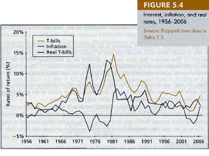
Do the historical rates of return we reviewed in the previous section, measured in nominal dollars, reflect the increase in our purchasing power? Inflation rate – the rate at which prices are rising, measured as the rate of increase of such indices as CPI or GDP deflator. Nominal interest rate – the interest rate in terms of nominal (not adjusted for purchasing power) dollars. Real interest rate – the excess of the interest rate over the inflation rate. The growth rate of the purchasing power derived from an investment. The relationship between these three factors may be summarized by the equations given below: • The growth factor of your purchasing power, 1+r Real interest Nominal rate interest rate Inflation rate Approximated relationship • Equals the growth factor of your money, 1+R Exact relationship • divided by the new price level, 1+i Approximate rule overstates the real value by the factor of 1+i, but is perfectly exact for continuous compounded rates.

Example 5. 6: Real Versus Nominal Rates If the interest rate on a one-year CD is 8%, and you expect inflation to be 5% over the coming year. 1. Calculate the real interest rate using approximated formula. 2. Calculate the real interest rate using exact formula. 3. By how many percent does the approximated formula overstate the expected real rate. Answers: 1. r = 8% - 5% = 3% 2. 3. Approximated formula overstates the expected real rate by only 0. 14%, or 14 b. p. To summarize about these issues: In interpreting the historical returns on various asset classes we must recognize that to obtain real returns on these assets, we must reduce the nominal returns by the inflation rate. In fact, while the return on the U. S. Treasury Bill usually is considered to be riskless, this is true only in regard to its nominal return. To infer the expected real rate of return on a T-bill, you must subtract your estimate of the inflation rate over the coming period. It is always possible to calculate the real rate after the fact. The future real rate, however, is unknown, and you need to rely on expectations. In other words, because future inflation is risky, the real rate of return is risky even if the nominal rate is risk-free.
 Nominal interest rate Expected")
Fischer Equation Real interest rate R = r + E(i) Nominal interest rate Expected Inflation rate Logic: Because investors should be concerned with their real returns – the increase in their purchasing power – we would expect that as inflation increases, investors will demand higher nominal rates of return on their investments. This higher rate is necessary to maintain the expected real return offered by an investment. Take a look on Figure 5. 4 you may see that periods of high inflation and high nominal interest rates generally coincide. Concept Check 5. 5 a. Suppose the real interest rate is 3% per year, and the expected inflation rate is 8%. What is the nominal rate of interest? b. Suppose the expected inflation rises to 10%, but the real rate is unchanged. What should we expect to happen to the nominal interest rate? Answers: a. R = r + E(i) => 3% = r + 8% => r = 5% b. R = r + E(i) => 3% = r + 10% => r = 7%

First steps of investment process generally consists of two decisions: 1. Asset allocation 2. Security selection In this and the next chapter we will talk generally with the asset allocation decision. Asset allocation – portfolio choice among broad investment classes. “How much of our money to allocate among different broad asset classes, such as bonds, stocks, precious metals, international or sovereign securities, etc. ” Most investment professionals consider asset allocation the most important part of the portfolio construction. The most fundamental decision of investing is the allocation of your assets: How much should you own in stock? How much should you own in bonds? How much should you own in cash reserves? . . . That decision [has been shown to account] for an astonishing 94% of the differences in total returns achieved by institutionally managed pension funds… There is no reason to believe that the same relationship does not also hold true for individual investors. John Bogle, at that time chairman of the Vanguard Group of Investment Companies

How will we proceed: 1. We will denote the investor’s portfolio of risky assets as P, and the risk-free asset as F. 2. We will assume for the sake of illustration that the risky component of the investor’s overall portfolio comprises two mutual funds: one invested in stocks and the other invested in longterm bonds. 3. For now we take the asset composition as given and focus only on the allocation between it and risk-free securities. When we shift wealth from the risky portfolio (P) to the risk-free asset, we don’t change the relative proportions of the various securities within the risky portfolio. Rather, we reduce the relative weight of the risky portfolio as a whole in favor of risk-free assets. An example of asset allocation Assume that total market value of an investment portfolio is $300’ 000 distributed as follows among risky and risk-free assets: Asset Risk prospects $ Amount Ready Assets money market fund Risk-free Vanguard S&P 500 Index Risky $113 400 Fidelity Investment Grade Bond Fund Risky $96 600 Total Market Value of portfolio $90 000 Ready Assets MMF (F) invests primarily in U. S. $300 000 Treasury securities Vanguard fund (V) is a passive equity fund that replicates the S&P 500 portfolio. Fidelity Investment Grade Bond Fund (IG) invests primarily in corporate bonds with high safety ratings and also in Treasury bonds.

Source: Vanguard Group site for personal investors https: //personal. vanguard. com

Source: Vanguard Group site for personal investors https: //personal. vanguard. com

Source: fundresearch. fidelity. com
 The holdings of the Vanguard and Fidelity shares")
Composition of the risky portfolio (P) The holdings of the Vanguard and Fidelity shares make up the risky portfolio, with 54% in V and 46% in IG. w. V = 113’ 400/210’ 000 = 0. 54 (Vanguard) w. IG = 96’ 600/210’ 000 = 0. 46 (Fidelity) The weight of the risky portfolio, P, in the complete portfolio (the entire portfolio including risky and risk-free assets) is denoted by y, and so the weight of the MMF is 1 -y. y = 210’ 000/300’ 000 = 0. 7 (risky asset, portfolio P) 1 -y = 90’ 000/300’ 000 = 0. 3 (risk-free assets, F) The weights of the individual assets in the complete portfolio (C) are: Vanguard Fidelity Portfolio P Ready Assets F Portfolio C 113'400/300'000 = 96'600/300'000 = 210'000/300'000 = 90'000/300'000 = 300'000/300'000 = 0. 378 0. 322 0. 700 0. 300 1. 000 Suppose the investor decides to decrease risk by reducing the exposure to the risky portfolio from 70% to 56%. • What would be the new composition of a portfolio? As a form you may use the table above. • What dollar amount of Vanguard and Fidelity shares we need to sell and what dollar amount of Ready Assets should we purchase to obtain this portfolio?

• What would be the new composition of a portfolio? As a form you may use the table above. Asset____ Vanguard Fidelity Portfolio P Ready Assets F Portfolio C $ Amount $90 720 $77 280 $168 000 $132 000 $300 000 % Weight 0, 302 0, 258 0, 560 0, 440 1, 000 Calculations: • Portfolio P = $300’ 000 × 0. 56 • Ready Assets F = $300’ 000 × 0. 44 • $ Amount Vanguard = $168’ 000 × 0. 54 • $ Amount Fidelity = $168’ 000 × 0. 46 • % Weight Vanguard = $90’ 720/$300’ 000 • % Weight Fidelity = $77’ 280/$300’ 000 • What dollar amount of Vanguard and Fidelity shares we need to sell and what dollar amount of Ready Assets should we purchase to obtain this portfolio? Calculations: • Vanguard shares to be sold = 113’ 400 – 90’ 720 = $22’ 680 $42’ 000 • Fidelity shares to be sold = 96’ 600 – 77’ 280 = $19’ 320 • Ready Assets shares to be purchased = 132’ 000 – 90’ 000 = $42’ 000 The key point is that we leave the proportion of each asset in the risky portfolio unchanged. Concept Check 5. 6 What will be the dollar value of your position in Vanguard and its proportion in your complete portfolio if you decide to hold 50% of your investment budget in Ready Assets?

Concept Check 5. 6 What will be the dollar value of your position in Vanguard and its proportion in your complete portfolio if you decide to hold 50% of your investment budget in Ready Assets? Answer: • $ value of the risky portfolio, P = 0. 50 × $300’ 000 = $150’ 000 • $ value of our position in Vanguard = 0. 54 × $150’ 000 = $81’ 000 • % proportion of Vanguard in complete portfolio = $81’ 000/$300’ 000 = 0. 27 = 27%

Let’s proceed to examine the risk-return combinations that result from various investment allocations between the risky and risk-free assets. Since we assume the composition of the optimal risky portfolio (P) already has been determined, the concern here is with the proportion of the investment budget (y) to be allocated to it. The remaining portion, (1 -y), will be invested in the risk-free asset. Assume that: • Rate of return on risky asset = r. P • Expected rate of return on risky asset = E(r) = 15% • Standard deviation of risky asset = σP = 22% • Rate of return on the risk-free asset = rf = 7% =>Risk premium on risky asset = E(r. P) - rf = 15% - 7% = 8% First of all let’s draw a graph with E(r) on the vertical axis and σP on the horizontal axis. Now let’s identify two extreme cases: 1. If you invest all of your funds into risky assets i. y = 1. 0 ii. E(r. C) = 15% iii. σC = 22% 2. If you invest all of your funds into riskfree asset i. y = 0 ii. E(r. C) = 7% iii. σC = 0%

Now consider more moderate choices 3. You invest equally in risky and risk-free assets i. y = 0. 5 ii. E(r. C) = 0. 5× 15% + 0. 5× 7% = 11% iii. σC = 0. 5× 22% + 0. 5× 0% = 11% We may see that when you reduce the fraction of the complete portfolio allocated to the risky asset by half, you reduce both the risk and the risk premium by half (8% VS 4%) The standard deviation of the complete portfolio will equal the standard deviation of the risky asset times the fraction of the portfolio invested in the risky asset. To generalize, the risk premium of the σC = yσP complete portfolio, C, will equal the risk premium of the risky asset times the The slope of the F-P line will be the Sharpe fraction of the portfolio invested in the risky ratio. asset.

Concept Check 5. 6 What are the expected return, risk premium, standard deviation, and ratio of risk premium to standard deviation for a complete portfolio with y = 0. 75? Answer: • E(r. C) = 0. 75× 15% + 0. 25× 7% = 11. 25% + 1. 75% = 13% • Risk premium = E(r. C) – rf = 13% - 7% = 5% • σC = 0. 75× 22% + 0. 25× 0% = 16. 5% = 0. 75× 22% • Note: don’t forget that we were talking about in this section was devoted to trade-off between a risky and a risk-free portfolios. The issue with a trade-off between two risky portfolios is a different thing.

Capital allocation line Plot of risk-return combinations available by varying portfolio allocation between a risk-free asset and a risky portfolio. We can rewrite our calculations for CAL as What about points on the line to the right of portfolio P in the investment opportunity set? Example 5. 7 Levered Complete Portfolio Suppose the investment budget is $300’ 000, and our investor borrows an additional $120’ 000 at a risk-free rate, investing the $420’ 000 in the risky asset. • what will be the “y”? • what will be the expected return, risk premium, standard deviation, and ratio of risk premium to standard deviation for a complete portfolio with the new “y”

Example 5. 7 Levered Complete Portfolio Suppose the investment budget is $300’ 000, and our investor borrows an additional $120’ 000 at a risk-free rate, investing the $420’ 000 in the risky asset. • what will be the “y”? • what will be the expected return, risk premium, standard deviation, and ratio of risk premium to standard deviation for a complete portfolio with the new “y” • y = $420’ 000/$300’ 000 = 1. 4 • E(r. C) = 1. 40 × 15 – 0. 4 × 7= 18. 2% = (420’ 000× 0. 15 -120’ 000× 0. 07)/300’ 000 • Risk premium = E(r. C) – rf = 18. 2% - 7% = 11. 2% • σC = 1. 40× 22% = 30. 8% • As you might have expected, the levered portfolio has both a higher expected return and a higher standard deviation than an unlevered position in the risky asset.

eat well VS sleep well • More risk averse investors will choose portfolios near F on the CAL above. • More risk-tolerant investors will choose portfolios near P. • Even more Risky investors will choose portfolios to he right of the point P The investor’s asset allocation choice also depends on the trade-off between risk and return. • If the Sharpe ratio increases, investors might well decide to take on riskier positions. One role of the professional financial adviser is to 1. present investment opportunity alternatives to clients 2. obtain an assessment of the client’s risk tolerance 3. help determine an appropriate complete portfolio

Passive strategy – investment policy based on the philosophy that securities are fairly priced and it avoids the costs involved in undertaking security analysis. To avoid the costs of acquiring information on any individual stock or a group of stocks, we may follow a “neutral” diversification approach. Here we select a portfolio which mirrors a broad market indices, such as S&P 500 or Russell 2000. Þ Thus, such strategies are also called indexing. Þ The rate of return on portfolio then replicates the return on the index. We call the capital allocation line (CAL) provided by one-month T-bills and a broad index of common stocks the capital market line (CML). Is it possible to use the CML on practice? => very hard, almost impossible

• Passive strategy is cheaper. Constructing an active portfolio is more expensive than constructing a passive one. Ex: index funds usually have the lowest operating expenses. • Free-rider benefit. Based on the efficient market hypothesis. • “Diversification is protection against ignorance. ” Warren Buffett. To summarize, • A passive strategy involves investment in two passive portfolios: • Virtually risk-free short-term T-bills (or a MMF), and • Fund of common stocks that mimics a broad market index • Recall that the CAL representing such a strategy is called a CML • Using Table 5. 5, we see that using 1926 -2006 data, the passive risky portfolio has offered an average excess return of 8. 4% with a standard deviation of 20. 4%, resulting in a reward to volatility ratio of 0. 41. • But might we expect the same numbers for the future?
Chapter 5 Risk and Return.pptx