Chapter 4 UTILITY MAXIMIZATION AND CHOICE Copyright

Chapter 4 UTILITY MAXIMIZATION AND CHOICE Copyright © 2005 by South-Western, a division of Thomson Learning. All rights reserved. 1

Objective: • Choosing among bundles of goods is a function of two things: (1) preferences, and (2) what you can afford • Last lecture: we studied a method to represent consumer’s preferences (1) • In this lecture, we will study (2) and how (1) and (2) are combined to study choice among bundles of goods 2

The Budget Constraint • What bundles of goods (X, Y) can the individual afford if he has £I and prices (px and py ) are independent of the quantity purchased? • Those for which: pxx + pyy I; • It is helpful to draw the combinations of (x, y) such that pxx + pyy =I. • We solve for y: y = I/py – (px /py) x • We can see that it is a straight decreasing line with slope – (px /py) • If x=0, y = I/py and if y=0, x= I/px 3

The Budget Constraint • If income changes, the budget constraint changes in parallel as the slope (ratio of prices) do not change • If prices change, then the slope also changes • See some examples in the board 4

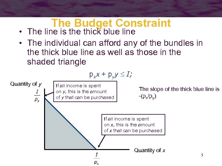The Budget Constraint • The line is the thick blue line • The individual can afford any of the bundles in the thick blue line as well as those in the shaded triangle pxx + pyy I; Quantity of y If all income is spent on y, this is the amount of y that can be purchased The slope of the thick blue line is -(px/py) If all income is spent on x, this is the amount of x that can be purchased Quantity of x 5

Starting to combine (1) and (2) • How are choices among bundles of goods done? • We assume that consumers will maximize utility among the bundles that they can afford 6

Optimal choice when the MRS is strictly decreasing • If the MRS is strictly decreasing then the indifference curve is convex • Using a graph, let’s study utility maximization (with convex indifference curves) subject to the consumer’s budget constraint 7

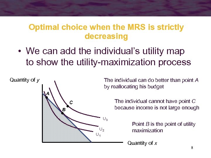Optimal choice when the MRS is strictly decreasing • We can add the individual’s utility map to show the utility-maximization process Quantity of y The individual can do better than point A by reallocating his budget A The individual cannot have point C because income is not large enough C B U 3 U 2 U 1 Point B is the point of utility maximization Quantity of x 8

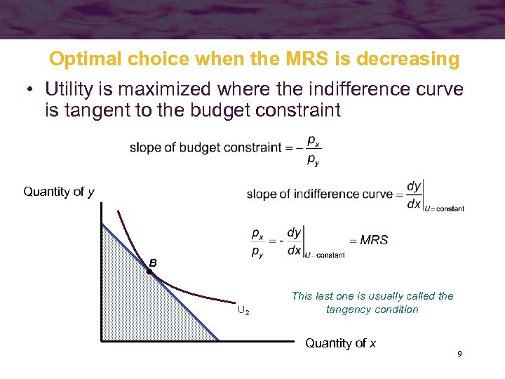Optimal choice when the MRS is decreasing • Utility is maximized where the indifference curve is tangent to the budget constraint Quantity of y B U 2 This last one is usually called the tangency condition Quantity of x 9

Optimal choice when the MRS is strictly decreasing • We call the MRS=ratio of prices the tangency condition • Verifying the tangency condition is a sufficient condition for a bundle to be an optimal choice, when the MRS strictly is decreasing • What? is the intuition behind the tangency condition? 10

A Numerical Illustration • Assume that the individual’s MRS = 1 – willing to trade one unit of x for one unit of y • Suppose the price of x = $2 and the price of y = $1 • The individual can be made better off – trade 1 unit of x for 2 units of y in the marketplace • So, it cannot be an optimal bundle if MRS is different from the ratio of prices 11

Maths for when MRS is strictly decreasing • Same as before but using mathematics… • We will see how the tangency condition comes up in the mathematical exercise • The individual’s objective is to maximize utility = U(x 1, x 2) subject to the budget constraint I = p 1 x 1 + p 2 x 2 • Set up the Lagrangian: L = U(x 1, x 2) + (I - p 1 x 1 - p 2 x 2 ) 12

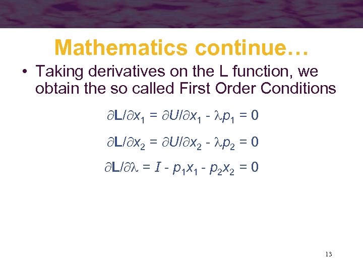Mathematics continue… • Taking derivatives on the L function, we obtain the so called First Order Conditions L/ x 1 = U/ x 1 - p 1 = 0 L/ x 2 = U/ x 2 - p 2 = 0 L/ = I - p 1 x 1 - p 2 x 2 = 0 13

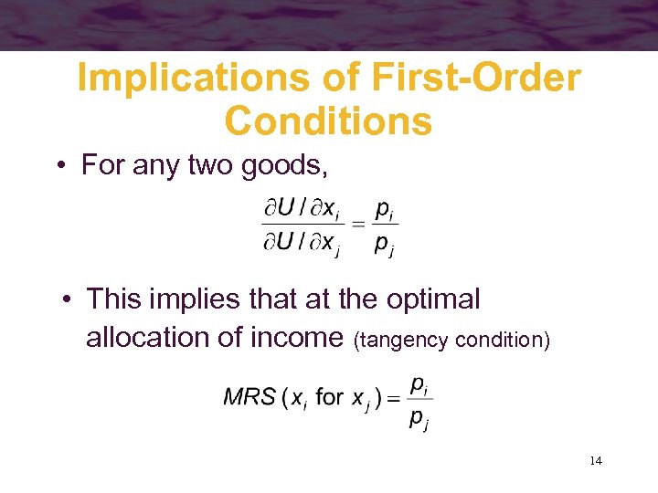Implications of First-Order Conditions • For any two goods, • This implies that at the optimal allocation of income (tangency condition) 14

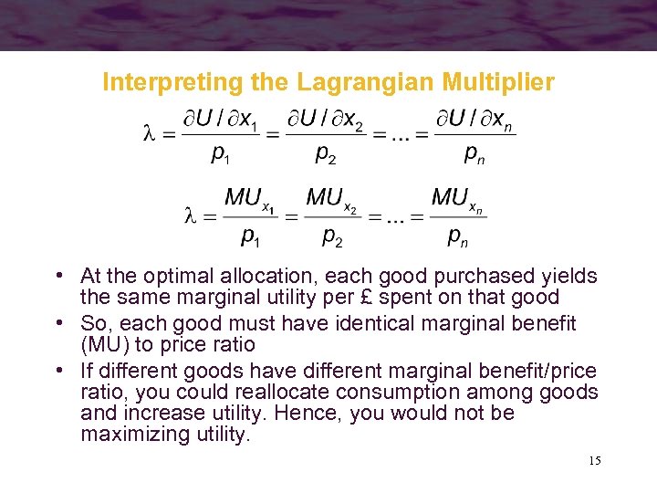Interpreting the Lagrangian Multiplier • At the optimal allocation, each good purchased yields the same marginal utility per £ spent on that good • So, each good must have identical marginal benefit (MU) to price ratio • If different goods have different marginal benefit/price ratio, you could reallocate consumption among goods and increase utility. Hence, you would not be maximizing utility. 15

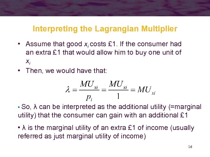Interpreting the Lagrangian Multiplier • Assume that good xi costs £ 1. If the consumer had an extra £ 1 that would allow him to buy one unit of xi • Then, we would have that: • So, λ can be interpreted as the additional utility (=marginal utility) that the consumer can gain with an additional £ 1 • λ is the marginal utility of an extra £ 1 of income (usually referred as just marginal utility of income) 16

Optimal choice when MRS is strictly decreasing • We said “Verifying the tangency condition is a sufficient condition for a bundle to be an optimal choice, when the MRS is decreasing” • So, it is not a necessary condition • This means that a bundle might be an optimal choice but might not verify the “tangency condition” even if the MRS is decreasing • This happens because of corner solutions (see next slide) – Corner solution: consumption zero of at least one good of the bundle – Interior solution: positive consumption of all the goods of the bundle 17

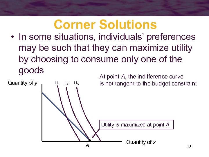Corner Solutions • In some situations, individuals’ preferences may be such that they can maximize utility by choosing to consume only one of the goods Quantity of y U 1 U 2 At point A, the indifference curve is not tangent to the budget constraint U 3 Utility is maximized at point A A Quantity of x 18

Optimal choice when MRS is no decreasing • So far, we have assumed that MRS is decreasing. Otherwise… • The tangency rule is necessary but not sufficient – That is the optimal choice (if it is interior) will verify the tangency rule but there will be bundles that verify the optimal rule but are not optimal choices • If MRS is not diminishing, then we must check second-order conditions to ensure that we are at a maximum 19

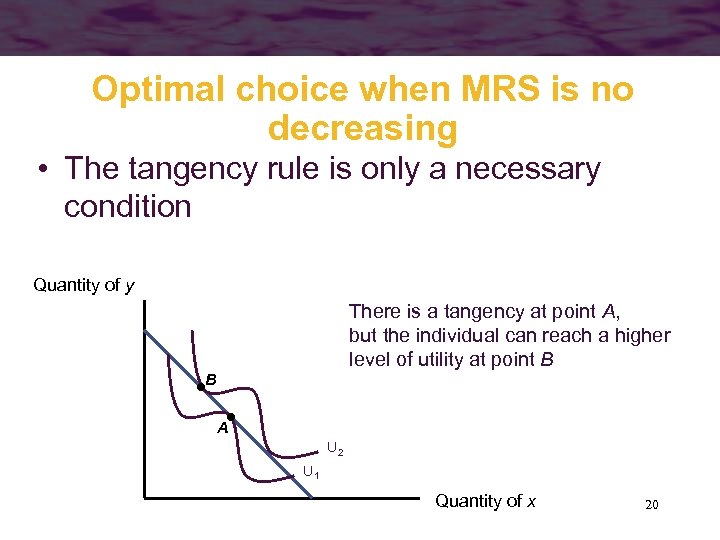Optimal choice when MRS is no decreasing • The tangency rule is only a necessary condition Quantity of y There is a tangency at point A, but the individual can reach a higher level of utility at point B B A U 2 U 1 Quantity of x 20

When does the tangency condition not work? • If the MRS is constant ( the indifference curves are straight lines), for instance: perfect substitutes • If either the indifference curves or budget constraint are non differentiable (have kinks). For instance: complements • In some cases, when the individual prefers to consume zero of one of the goods. When this happens, the solution is called a corner solution • Graphical analysis is usually very useful 21

Roadmap to compute optimal choice when prices are constant, and utility function is differentiable • A) Compute the utility at all possible corner solutions • B) Compute optimal interior bundles by solving the optimization using the Langrangian to obtain the tangency condition (alternatively, apply the tangency condition directly) • C) if MRS is strictly decreasing, solutions in B are local optima. Compare them with those in A) and obtain the optimal choice • D) if MRS is not strictly decreasing, you might have found some bundles that are not even local maxima. Apply SOC to find the local optima. If you get more than one local optima, find out which is the one that give more utility. Compare it with the ones obtained in A 22 • E) Graphical analysis usually helps !

Example with Cobb-Douglas Utility U(x, y) = x y Budget constraint: I = pxx + pyy Corner solutions cannot be optimal (U=0) Budget constraint is standard, it does not have kinds • Utility function does not have kinks • • • It is easier if we take ln • U= ln(x)+ ln(y) • MRS=y/x (-ratio of marginal utilities, see prev. lecture) is strictly decreasing in x • We can apply the maths and the tangency 23 condition is necessary and sufficient

Example with Cobb-Douglas Utility function U= ln(x)+ ln(y) Budget constraint: I = pxx + pyy • Setting up the Lagrangian: L = ln(x)+ ln(y) + (I - pxx - pyy) • First-order conditions: L/ x = /x - px = 0 L/ y = /y - py = 0 L/ = I - pxx - pyy = 0 24

Cobb-Douglas utility function • First-order conditions imply: y/ x = px/py • We obtain the tangency condition as a result of solving the optimization problem… • Substituting into the budget constraint: I = pxx + [ / ]pxx = (( + )/ )pxx 25

Cobb-Douglas utility function • Solving for x yields X*=( /( + ))I/px • Substituting in the budget constraint, and solving for y, it yields: Y*=( /( + ))I/py • If corner solutions were possible, we would have to compare these solutions with the corner solutions and see which gives more utility • The percent of his income that the individual dedicates to each good is fixed and given by and • This might not be realistic… CES does not have this 26 property. We will use an exercise with CES

Example with perfect complements • U(x, y) = Min(x, 4 y) • Tangency condition will not hold, due to kinks in indifference curves. Do not use standard optimization technique but graphical analysis • The person will choose only combinations for which x = 4 y (use board…) • This means that I = pxx + pyy = pxx + py(x/4) I = (px + 0. 25 py)x 27

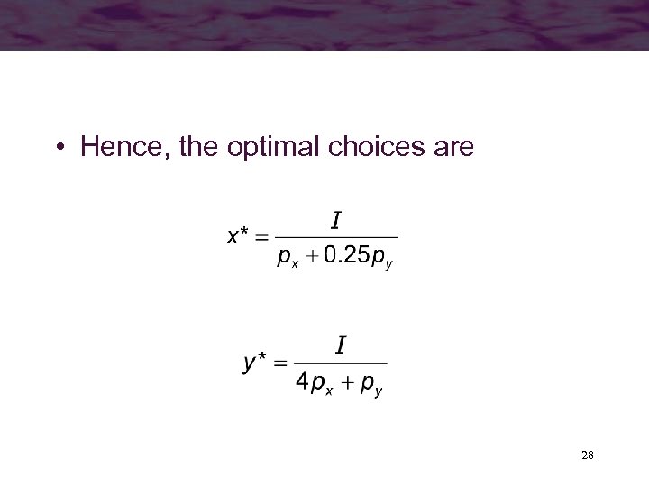• Hence, the optimal choices are 28

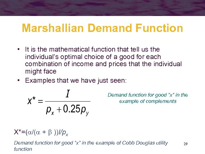Marshallian Demand Function • It is the mathematical function that tell us the individual’s optimal choice of a good for each combination of income and prices that the individual might face • Examples that we have just seen: Demand function for good “x” in the example of complements X*=( /( + ))I/px Demand function for good “x” in the example of Cobb Douglas utility function 29

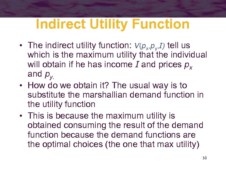Indirect Utility Function • The indirect utility function: V(px, py, I) tell us which is the maximum utility that the individual will obtain if he has income I and prices px and py. • How do we obtain it? The usual way is to substitute the marshallian demand function in the utility function • This is because the maximum utility is obtained consuming the result of the demand function because the demand functions are the optimal choices (the one that max utility) 30

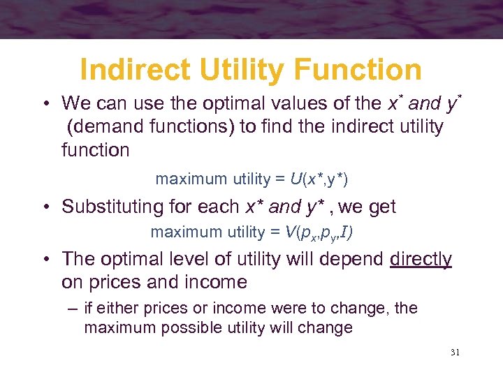Indirect Utility Function • We can use the optimal values of the x* and y* (demand functions) to find the indirect utility function maximum utility = U(x*, y*) • Substituting for each x* and y* , we get maximum utility = V(px, py, I) • The optimal level of utility will depend directly on prices and income – if either prices or income were to change, the maximum possible utility will change 31

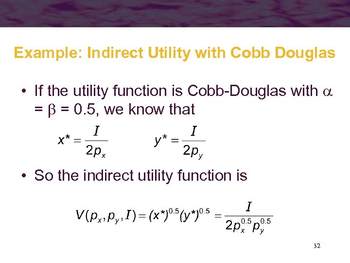Example: Indirect Utility with Cobb Douglas • If the utility function is Cobb-Douglas with = = 0. 5, we know that • So the indirect utility function is 32

Economic policy: taxing specific goods or taxing general purchasing power? • The government asks for your advice: is it best to tax income or specific goods? • The answer to this question is called the lump sum principle 33

The Lump Sum Principle • For the same amount of taxes collected, taxes on an individual’s general purchasing power are superior to taxes on a specific good – an income tax allows the individual to decide freely how to allocate remaining income – a tax on a specific good will reduce an individual’s purchasing power and distort his choices – Study the graph in pg. 107 in the book. Be sure that you understand footnote 8 !! 34

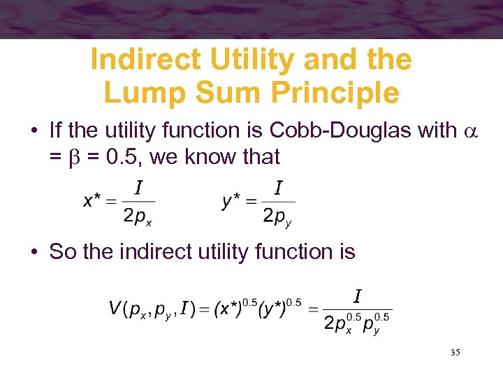Indirect Utility and the Lump Sum Principle • If the utility function is Cobb-Douglas with = = 0. 5, we know that • So the indirect utility function is 35

Indirect Utility and the Lump Sum Principle • px=1, py=4, I=8. Indirect utility V=2 • If a tax of £ 1 was imposed on good x – the individual will purchase x*=2 – indirect utility will fall from 2 to 1. 41 • An equal-revenue tax will reduce income to £ 6 – indirect utility will fall from 2 to 1. 5 36

Qualifying the Lump Sum Principle • In the above discussion, we have assumed that individuals will work the same independently of the income tax • If individuals work less because income tax is higher, it might be preferable to tax some goods rather than increasing income tax… • To study this, we need a more complicated model where individuals also choose how much to work, hence, their income 37

Expenditure Minimization • Another way of studying consumer’s optimal choices • Minimize expenditure subject to obtain a given level of utility – Optimal bundle of goods: the one that minimizes the required expenditure to achieve a given level of utility – this means that the goal and the constraint have been reversed 38

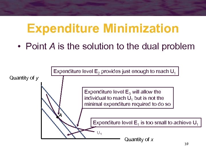Expenditure Minimization • Point A is the solution to the dual problem Quantity of y Expenditure level E 2 provides just enough to reach U 1 Expenditure level E 3 will allow the individual to reach U 1 but is not the minimal expenditure required to do so A Expenditure level E 1 is too small to achieve U 1 Quantity of x 39

Expenditure Function • The expenditure function shows the minimal expenditures necessary to achieve a given utility level for a particular set of prices minimal expenditures = E(px, py, U) • The expenditure function and the indirect utility function are inversely related – both depend on market prices but involve different constraints 40

Expenditure Minimization • The individual’s problem is to choose x, y, to minimize total expenditures = E = pxx + pyy subject to the constraint utility = U 1 = U(x, y) • The optimal amounts of x, y will depend on the prices of the goods and the required utility level 41

Equivalence • Solve the standard problem with prices px, py, and I: MAX utility subject to budget constraint. Say that the optimal utility is U 1 • If we solve the Min Expenditure, subject to achieving utility U 1 • Then, the optimal bundles of goods are the same in both problems, and the optimal expenditure in the second problem is I • See this with the graph… 42

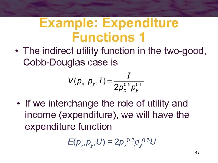Example: Expenditure Functions 1 • The indirect utility function in the two-good, Cobb-Douglas case is • If we interchange the role of utility and income (expenditure), we will have the expenditure function E(px, py, U) = 2 px 0. 5 py 0. 5 U 43

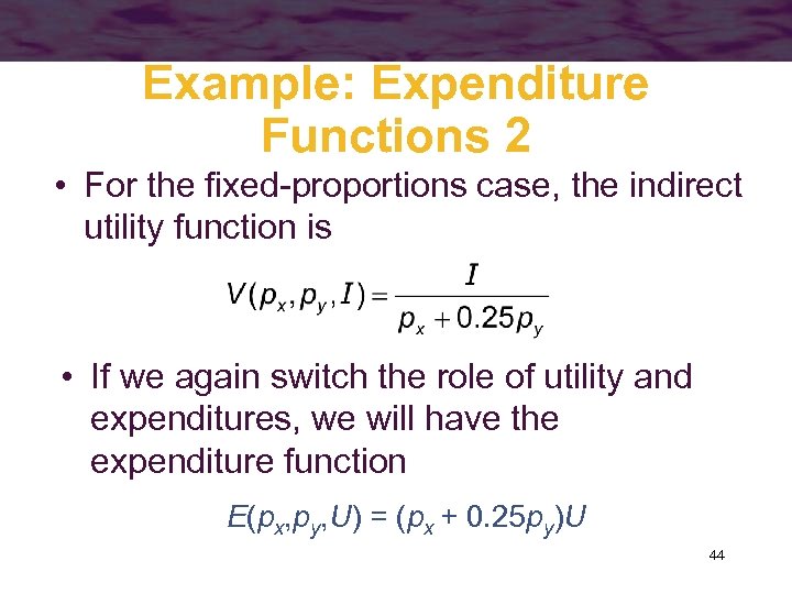Example: Expenditure Functions 2 • For the fixed-proportions case, the indirect utility function is • If we again switch the role of utility and expenditures, we will have the expenditure function E(px, py, U) = (px + 0. 25 py)U 44

Properties of Expenditure Functions • Homogeneity – a doubling of all prices will precisely double the value of required expenditures • homogeneous of degree one • Nondecreasing in prices – E/ pi 0 for every good, i • Concave in prices 45

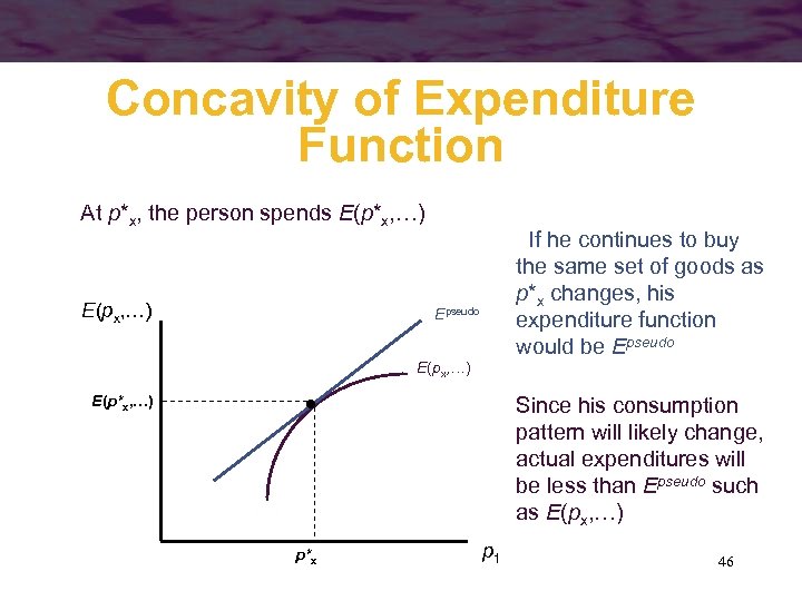Concavity of Expenditure Function At p*x, the person spends E(p*x, …) E(px, …) If he continues to buy the same set of goods as p*x changes, his expenditure function would be Epseudo E(px, …) E(p*x, …) Since his consumption pattern will likely change, actual expenditures will be less than Epseudo such as E(px, …) p*x p 1 46

Important Points to Note: • Consumer’s optimal choice: – spend all available income – choose a commodity bundle such that the MRS between any two goods is equal to the ratio of the goods’ prices (if MRS is strictly decreasing, there are no kinks and no corner solutions) – This is called the tangency condition 47

Important Points to Note: • The individual’s optimal choices implicitly depend on the parameters of his budget constraint – choices observed will be implicit functions of prices and income – utility will also be an indirect function of prices and income 48

Important Points to Note: • The dual problem to the constrained utility-maximization problem is to minimize the expenditure required to reach a given utility target – yields the same optimal solution as the primary problem – leads to expenditure functions in which spending is a function of the utility target and prices 49